Week 4.1 - Solving second order ODEs

Simple Pendulum

Aim: To write MATLAB script to solve second-order ODE equation of simple pendulum motion with damping. To create the animation of the motion of the pendulum.

Introduction:

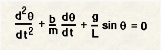
The equation of motion of a simple pendulum with damping is as follows

----------- eq.1

The above equation is a second-order differential equation. We will simplify the equation into two first-order differential equations.

We assume

`(d theta)/(dt) = theta_1` and ---------- eq.2

`(d^2 theta)/(dt^2) = (d theta_1)/dt = theta_2`

on substituting the above equations 2 and 3 in equation 1:

`theta_2 = -(b/m)*theta_1 -(g/L)sin(theta)` --------------- eq.3

`d/dt [[theta_1], [theta_2]] = [[theta_2],[-(b/m)theta_1 -(g/L)sin(theta)]]`

We will create a function which will represent this set of ODEs.

For this project,

Damping coefficient b = 0.05

Mass of the pendulum m = 1kg

Length of the pendulum L = 1m

Acceleration due to gravity g = 9.81 m/s^2

We will use the ode45 solver in this program to solve ODEs. The syntax for ode45 is as follows

[Time, Solution Vector] = ode45(@(Input) Ode Function/Equation Definition, Time Span, Initial Condition)

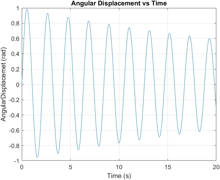
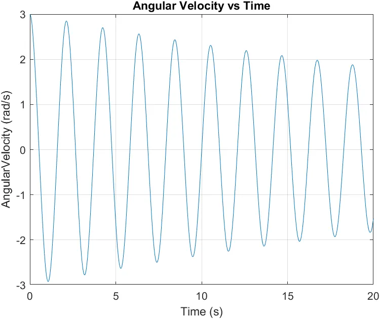
The solution vector obtained from the ode45 solve contains angular displacement and angular velocity of a pendulum with respect to time.

Time span will be 0 to 20 seconds

Using data on angular displacement, animation of the motion of the pendulum is created.

Main Program:

clear all
close all
clc

%% Inputs

%Constants
b= 0.05 ;       % Damping Coefficeint
g= 9.81;         % Acceleration due to Gravity
L=1;            % Length of the Pendulum
m=1;          % Mass of the Pendulum

% Initial condition 
theta_initial = [0;3];   % Angular Displacement | Angular Velocity

% Time Span
time_span = linspace(0,20,800);

%% Solution 
% For solving the ODE of equation of simple pendulum we use ode45 solver 
% Syntax for solving pendulum equation using ode45 solver is
% [Time, Theta_solution] = ode45(@(Input) Ode_Function/Equation_Defination, Time_Span, Initial_Condition)

[t, theta_solution] = ode45(@(t,theta_initial) pendulum(t,theta_initial,b,g,L,m),time_span,theta_initial);

Angular_Displacement = theta_solution(:,1);
Angular_Velocity = theta_solution(:,2);

% PLot for Angular Displacement vs Time
figure(1)
plot(t,Angular_Displacement)
title("Angular Displacement vs Time")
xlabel("Time (s)")
ylabel("AngularDisplacemet (rad)")
grid on

% PLot for Angular Velocity vs Time
figure(2)
plot(t,Angular_Velocity)
title("Angular Velocity vs Time")
xlabel("Time (s)")
ylabel("AngularVelocity (rad/s)")
grid on

%% Ploting and Animation the Motion of the Pendulum

x =  -L*sin(Angular_Displacement);          % x coordinates of the pendulum bob
y =  -L*cos(Angular_Displacement);          % y coordinates of the pendulum bob


for i = 1:length(Angular_Displacement)

   figure(3)
   hold on
    plot([-0.5 0.5],[0 0],'k-','LineWidth',10)    % Rigid wall that supports the Pendulum 
    plot([0 x(i)],[0 y(i)],'r-','LineWidth',3)    % Pendulum
    plot(x(i),y(i),'y.','MarkerSize',90)          % Pendulum Bob
       
    axis([-2 2 -2 2])
    grid on
   hold off
    M(i)=getframe(gcf);              % Creating an array which will store each frame of plots
   clf                              % To clear the current figure
end

videofile= VideoWriter("Pendulum.avi","Uncompressed AVI");  % Creating .avi file for the anuimation
open(videofile)
writeVideo(videofile,M);        % Stiching the frame present in M array into a video file
close(videofile)

Function:

%This  function represents the ODE equation of motion of simple pendulum
%with damping
%The following equation is results of converting Second order ODE to First
%order ODE.
function [d_theta_dt] = pendulum_equation(t,theta_solution,b,g,L,m)

theta1 = theta_solution(1);               % Theta1 represents angular displacement
theta2 = theta_solution(2);               % Theta2 represents the angular velocity

d_theta1_dt = theta2;
d_theta2_dt = -b/m*theta2 - g/L*sin(theta1);

d_theta_dt = [d_theta1_dt;d_theta2_dt];    % Creating a column array that represents solution vector

end

Output:

Conclusion:

Created the animation of motion of pendulum with damping by solving the ODE using ode45 solver in the MATLAB.