Week 4 - CHT Analysis on Exhaust port

CONJUGATE HEAT TRANSFER ANALYSIS ON EXHAUST PORT

AIM: - To simulate and analyze conjugate heat transfer analysis on the exhaust port.

THEORY: -

Conjugate Heat Transfer refers to the combination of conductive heat transfer in solid and convective heat transfer of fluid. Predominantly, in most engineering applications, we observe conjugate heat transfer where heat is been transferred between solid-fluid interactions. It becomes important to analyze conjugate heat transfer for the effective design of heat transfer devices like heaters, coolers, heat exchangers, etc.

Conjugate heat transfer is a complex yet effective heat transfer mechanism. Due to its effectiveness and wide application, it is important to study about conjugate heat transfer. We can find applications of conjugate heat transfer in the fields like automobiles, power plants, electrical and electronic devices, heating, ventilation and air conditioning system, etc.

PROCEDURE: -

WORKBENCH PROJECT

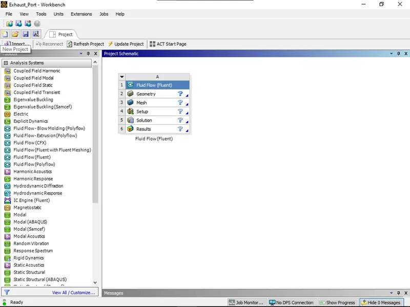
Start ANSYS Workbench and drag and drop Fluid Fluent into the main window and save it as Exhaust_Port.

Geometry with ANSYS Space Claim

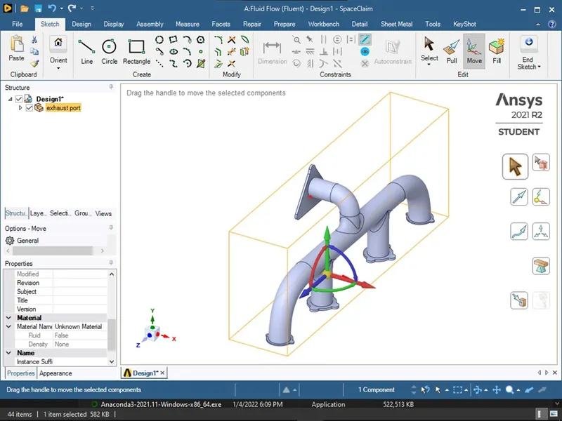
-Double Click on Geometry to open ANSYS Space Claim. Drag Drop the Exhaust Port model file on the Space Claim workspace in order to import the file.

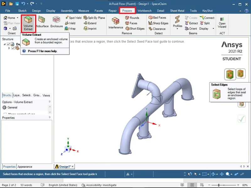
- Click on Prepare--> Volume Extract to extract the fluid volume inside the exhaust port.

-Click on Select Edge icon and select the inlet edges and outlet edge. Click on Right icon to complete the task.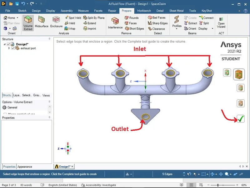

-There are chances of creation of non-conformal mesh between the interface of fluid and solid volume.

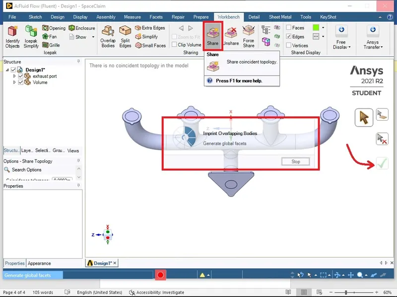
-For good intersection between solid and fluid volume we need to enable share topology. Make sure that all the component are present in single component. Click on Workbench--> Share to prepare conformal mesh. Click on Right icon to complete the task

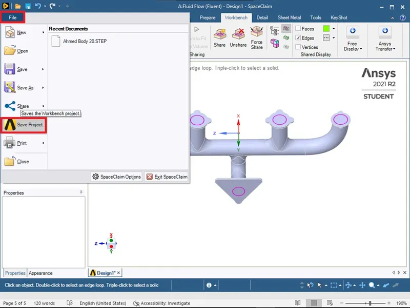
-Click on File --> Save Project to save the project and close the Space Claim.

MESHING IN ANSYS MESHING

-Double click on Mesh to open ANSYS Meshing.

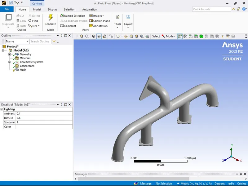
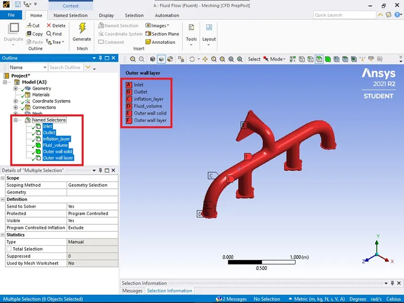
-Assign the Name for the faces of the Exhaust Port. Select the face by clicking on the face and press ‘N’ and type the face name.

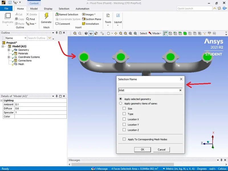
- Repeat the same step for all faces of Exhaust Port.

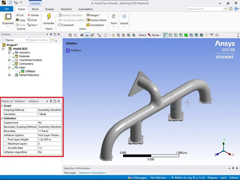
-In Outline tab, Right click on Mesh--> Insert -->Inflation. In Detail of ‘Inflation‘ tab, specify Named Selection in Scope Method tab. Specify Fluid Volume in Named Selection tab.

- Specify Named Selections in Boundary Scoping Method Tab. Specify Boundary as inflation layer Specify First Layer Thickness in Inflation Option tab. Specify 1.2e-03m as First Layer Height, 5 as Maximum Layer and 1.2 as Growth Rate.

-In Outline tab, Right click on Mesh--> Insert--> Sizing. In the Details of ‘Sizing’ tab, specify Named Selection for Scoping Method tab, specify Outer wall solid for Named Selection, specify 9e-02 as Element Size. Make sure to opt for Capture Curvature.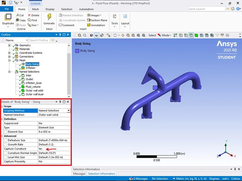

- Click on Generate icon to generate the mesh.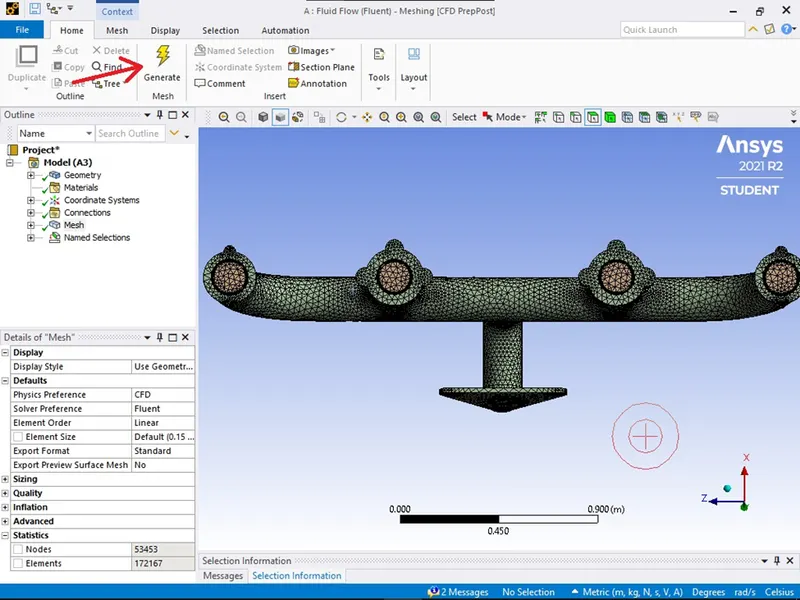

-File--> Save Project to save the project and close the ANSYS Meshing.

-In WorkBench, Right click on Mesh and Click on Update to update the Mesh details.

SETUP WITH ANSYS FLUENT

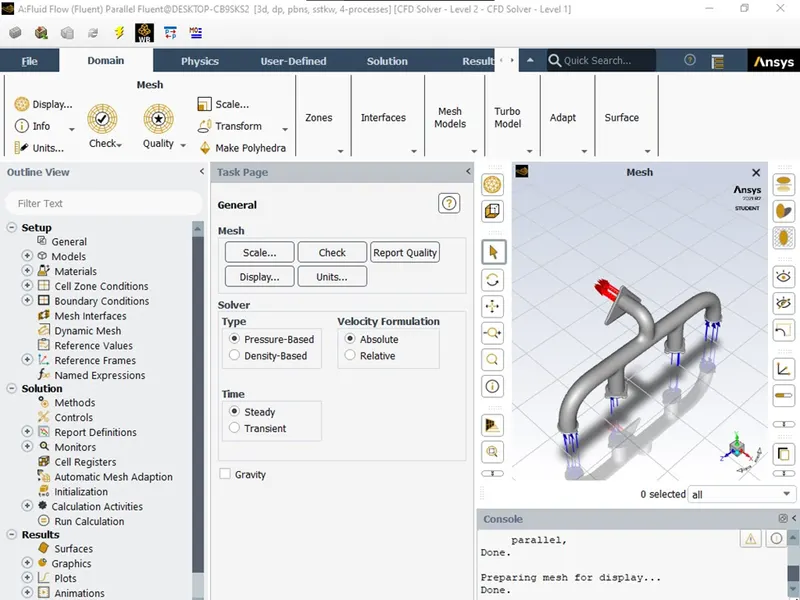
-In the WorkBench, click on setup to open ANSYS Fluent.

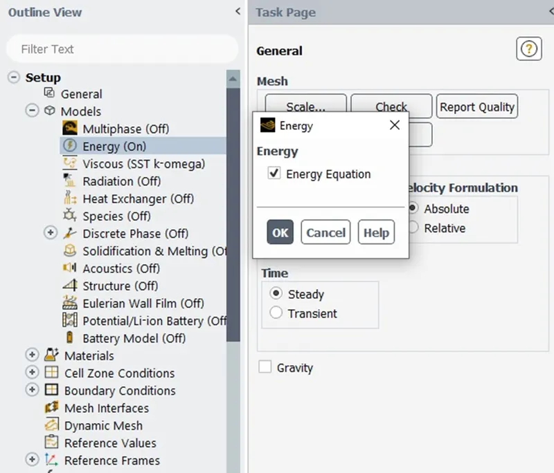
-In the Outline View tab, click on Model--> Energy, and tick the Energy Equation and click on OK.

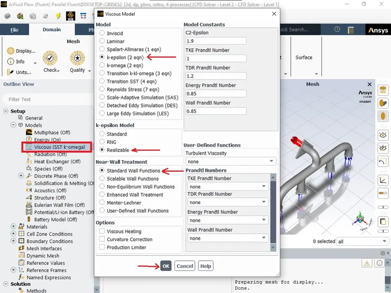
-Click on Model --> Viscous to setup the viscous model. Select k-epsilon model with Realizable and Standard Wall Function for Near-Wall Treatment.

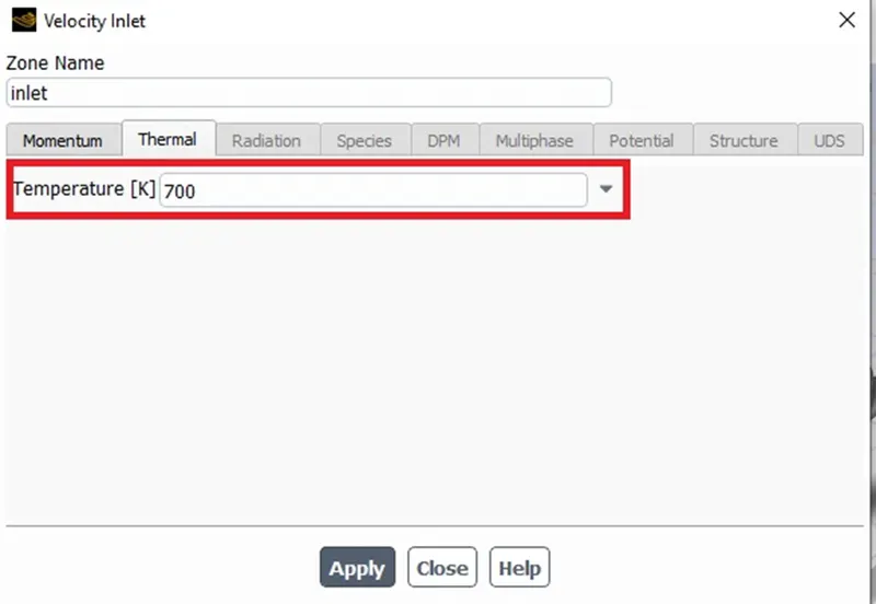
-To setup Inlet boundary Condition, click on Boundary Condition --> Inlet and Specify velocity as 5 m/s and temperature as 700 K.

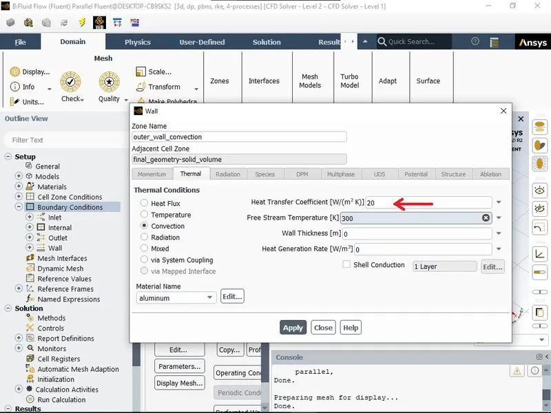
-Similarly for Wall boundary condition, click on Wall --> outer_wall_layer and Select Convection for Thermal Condition. Specify Heat Transfer Coefficient as 20.

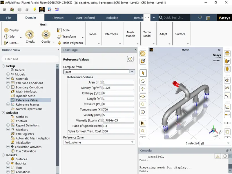
-Opt for Inlet for Compute From Tab in Reference Value Tab.

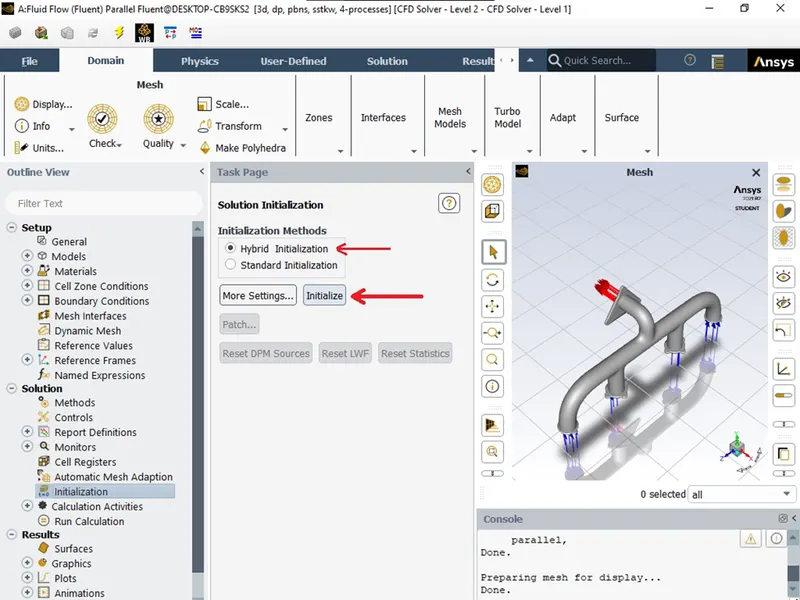
- For Solution Initialization, select Hybrid Initialization and click on Initialize.

-Click on Run Calculation and specify the Number of Iterations as 300. Click on Calculate.

RESULTS AND OUTCOME

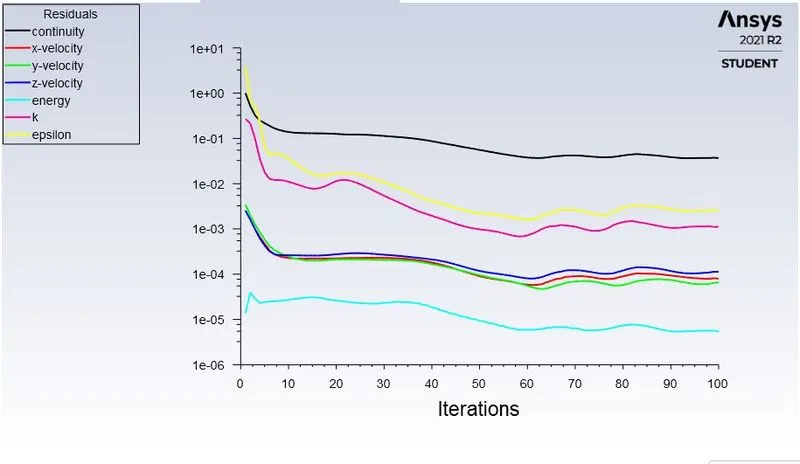
Residual Plot After 100 iterations

Area-Averaged temperature plot

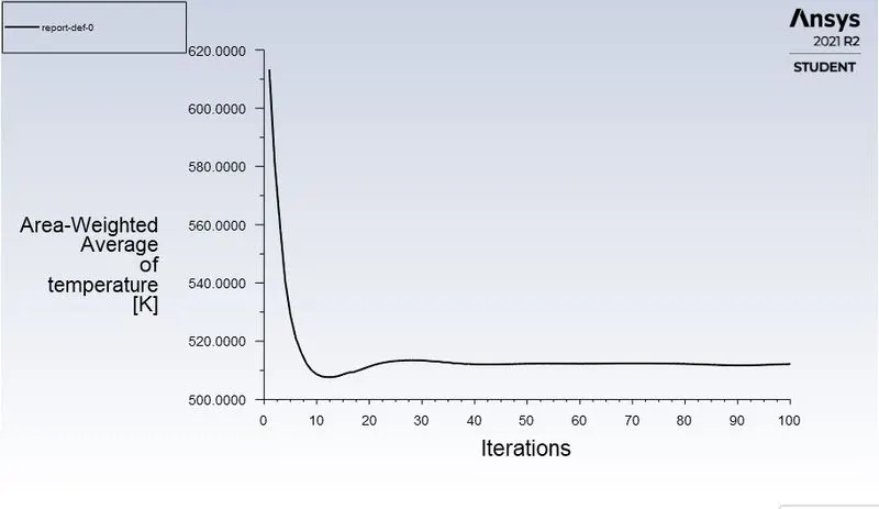
It is clear from the plot that it attains a steady state after about 30 iterations.

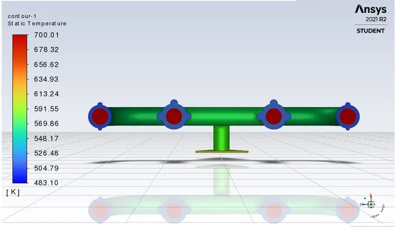
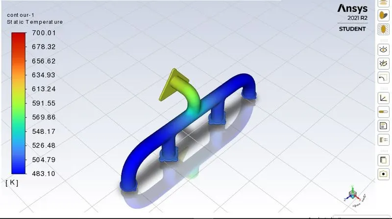
Temperature Contour

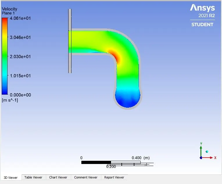
Velocity Contour

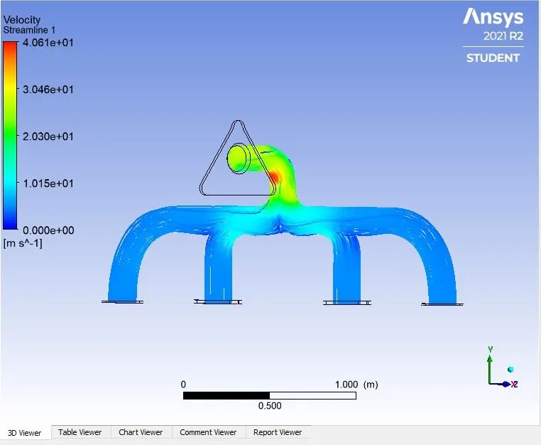
Streamlines

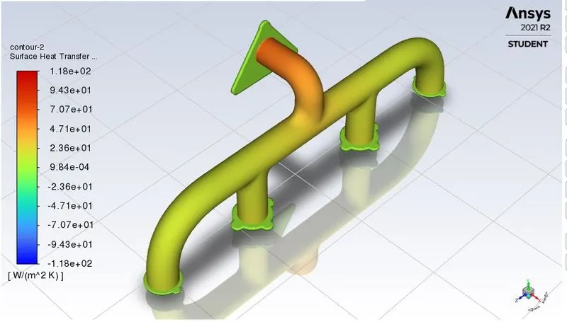
Contour for Wall Heat Transfer Coefficient

Factors affecting accuracy of prediction of heat transfer coefficient

Conjugate Heat Transfer Simulation performed in the computer are numerical simulations that can depict the actual event accurately but not exactly. The accuracy of a simulation depends on many parameters that can be improved by

• Refining the mesh and increasing the mesh quality.
• Adding Inflation layer near the boundary interface. Increasing mesh quality near the boundary interface will help in accurately capturing the phenomenon near the boundaries.

Analytically we can determine the heat transfer coefficient using the Dittus-Boelter correlation which is

h = (k*Nu)/D

Where k is the thermal conductivity of the fluid

D is the pipe diameter

Nu is Nusselt number

Further Nusselt number is calculated using the relation below

Nu = 0.023*Re*Pr

Where Re is Reynold’s Number

Pr is Prandtl Number

On putting all those values in the equation we will obtain the analytic value of the heat transfer coefficient. By comparing the analytical value with the predicted simulation value we can evaluate the accuracy of the simulation.

CONCLUSION

From the plots, contours, and results of the simulation, it is evident maximum heat transfer is at the bend near the exit port. Due to mass conservation velocity near the outlet is increase leads to an increase in Reynold’s Number making the flow turbulent. Flow is most turbulent near the bent near outlet port causes maximum heat transfer at the bent.

It can be concluded from the above simulation that the maximum and effective heat transfer flow should be turbulent.