Week 3: Flow over a backward facing step
Flow over a backwards-facing step
Aim: To simulate flow over a backwards-facing step using CONVERGE for three different mesh sizes. Post-process the results obtained from the simulation using Paraview and compare the results.
Theory:
Backwards facing step problem is a classic example to observe and understand the separation, recirculation, and reattachment of the flow. It is a basic model that involves the most important features of a separated flow: free shear flow separation, vortex evolution and re-attachment.
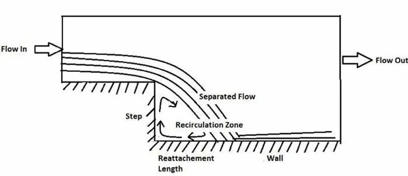
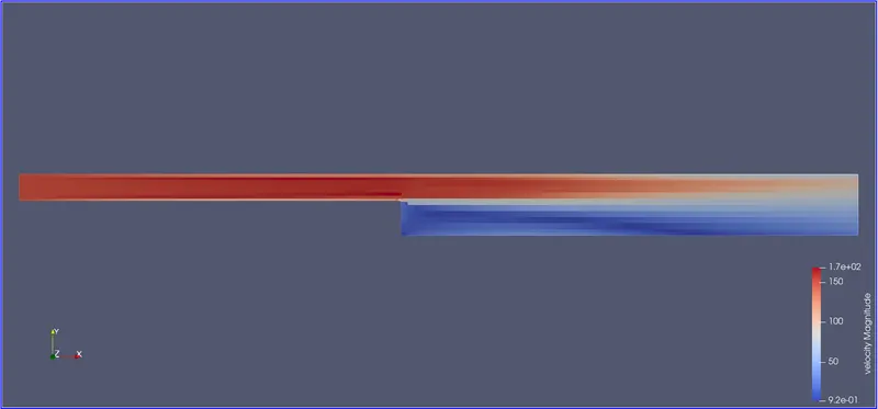
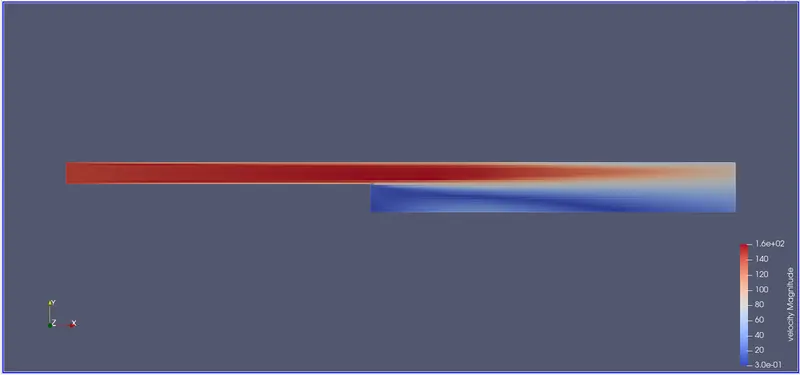
When a fully developed flow enters the domain and reaches the step, a pressure gradient exists due to an increase in cross-section, leading to flow separation. The flow detaches from the upper bottom wall and re-attaches to the lower bottom wall. In between a recirculation zone is formed.
A study of the backwards-facing step problem helps in analysing practical applications in internal flow systems like diffusers, combustors, and external flows like flow around aerofoil, aerodynamics of building and automobiles, etc.
Procedure:
Pre-processing:
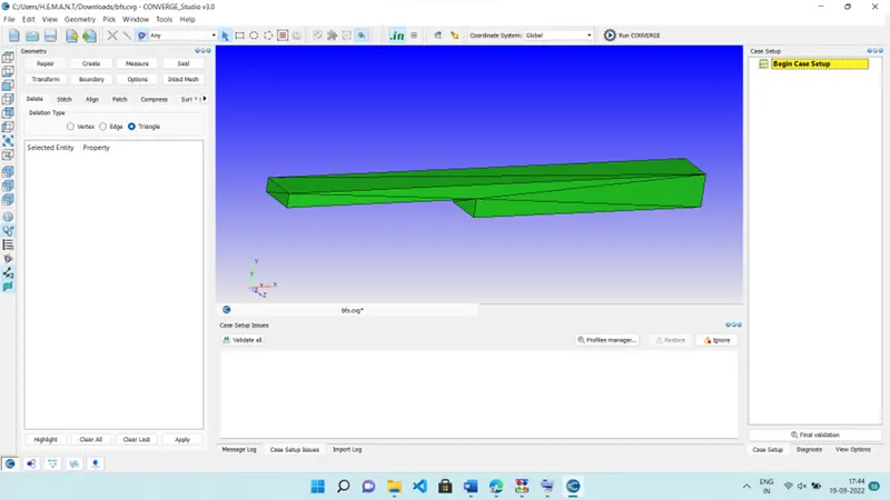
-Open the CONVERGE Studio. Import and load the .stl file (geometric model).
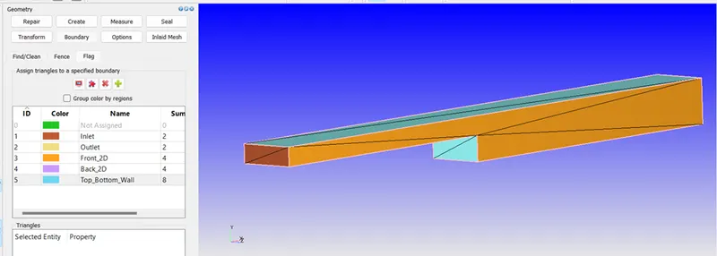
-Specify the boundaries to the geometry.
Simulation Set-up:
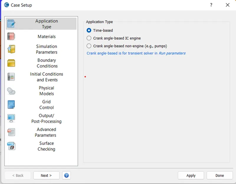
-To perform the simulation, select the Time-Based in the Application type. Click on apply and Done.
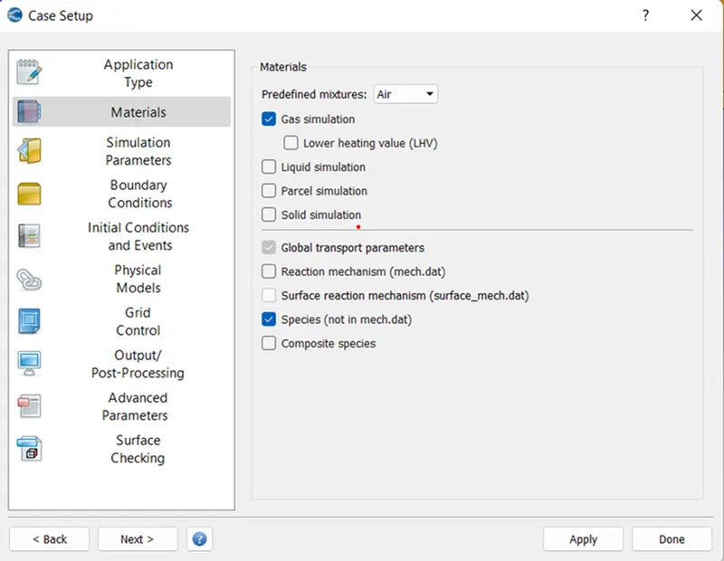
-For the Material, select ‘Air’ as Pre-Defined mixtures with the check on Gas simulation and Species.
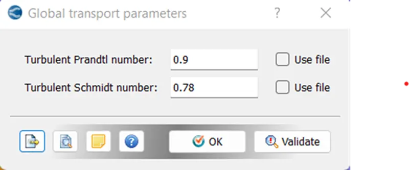
-For the Global transport parameter, specify the Turbulent Prandtl number as 0.9 and the Turbulent Schmidt number as 0.78. Click on Ok and Validate
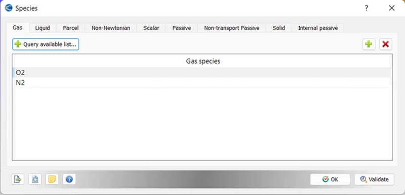
-For the Species, click on the ‘Plus’ symbol to add new species. Since this simulation is a gas simulation, we will add N2 and O2 in the Gas tab.
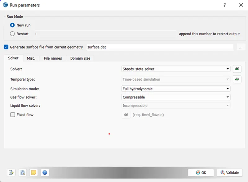
-For the Run Parameters, in the Solver tab specify the Solver as Steady-State Solver, Simulation mode as Full-hydrodynamic, and Gas flow solver as Compressible.
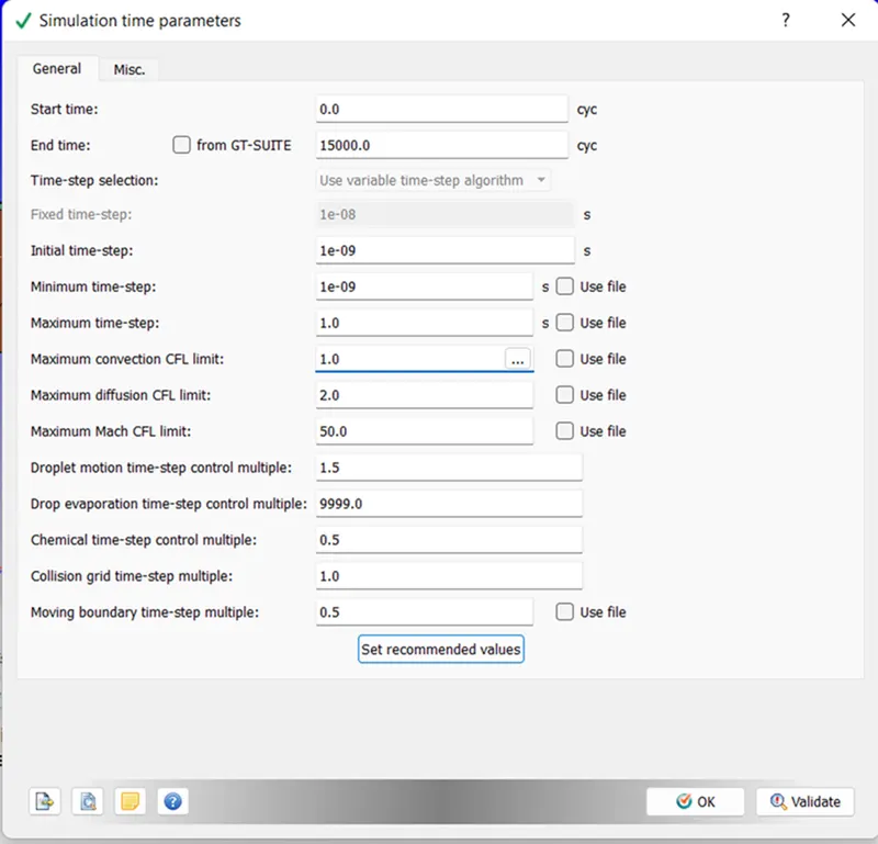
-For the Simulation Time Parameter, specify the details as shown in the following image.
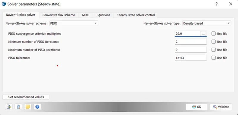
-For the Solver Parameter [Steady-State], use the Density-Based Navier-Stokes solver type. In the Equations tab, make sure that the precondition is set to none for all the equations.
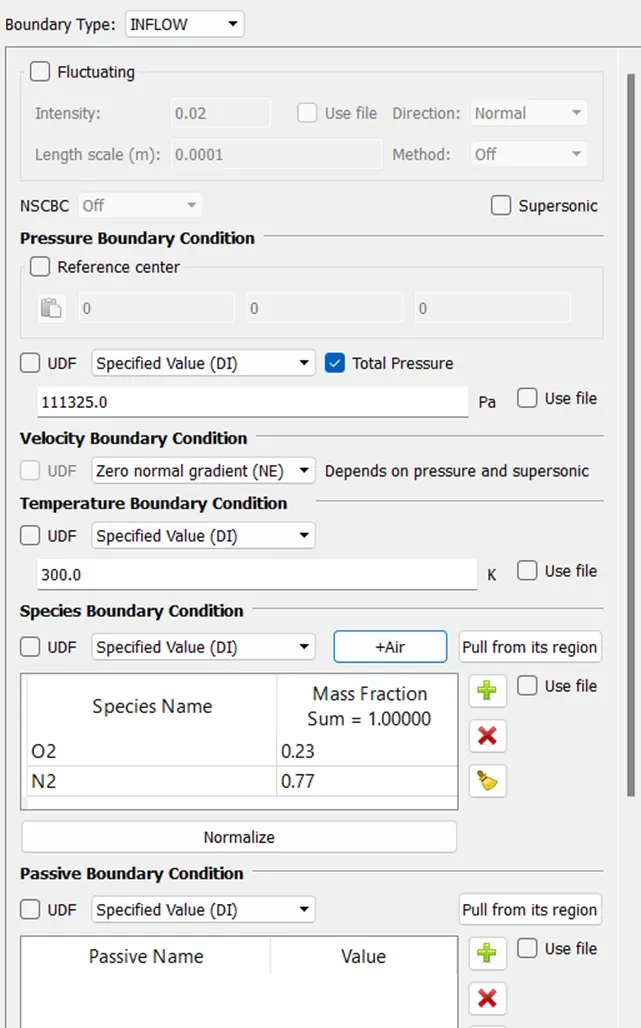
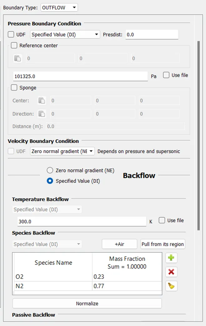
-Boundary Conditions are shown in the image
Inlet
Outlet
-Top and Bottom Wall:
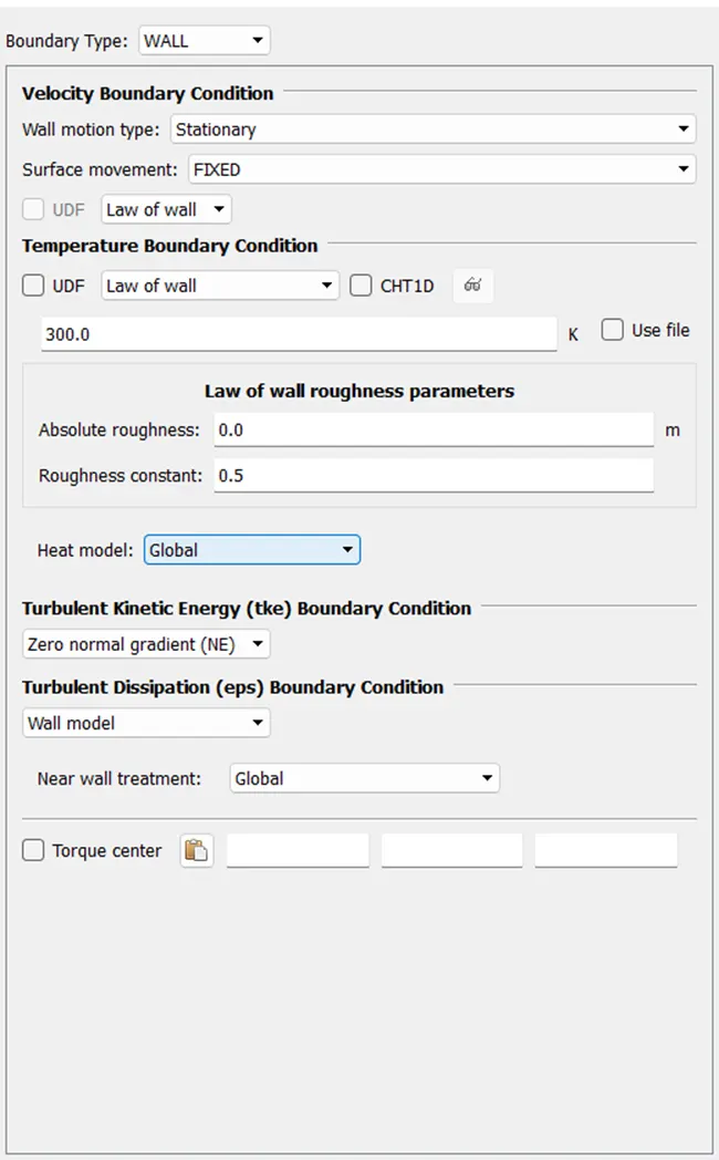
-Front and Back Walls:

-Steady-State monitor helps in observing the data obtain from simulation. Create a steady-state monitor for Avg. velocity. A velocity monitor is a setup with tolerance to observe the convergence of the result.
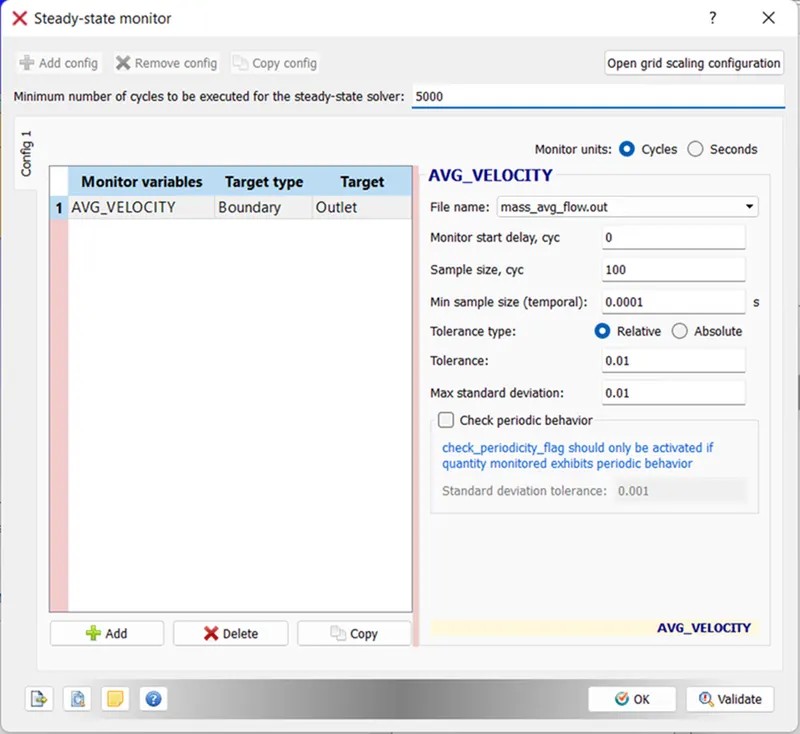
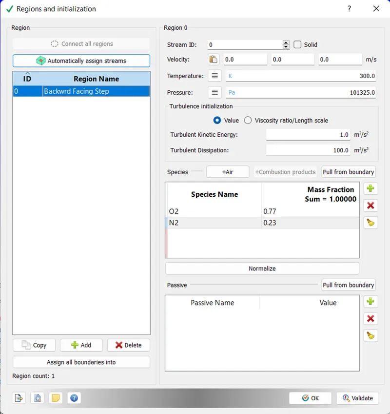
-In the Region and Initialization tab, Create the region/volume where the fluid will flow. Specify mass fraction for O2 as 0.77 and N2 as 0.23.
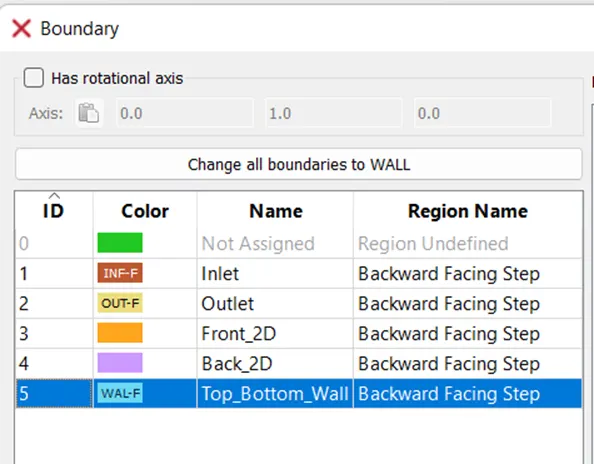
-To assign this region to all the boundaries click on the ‘Assign all boundaries into’.
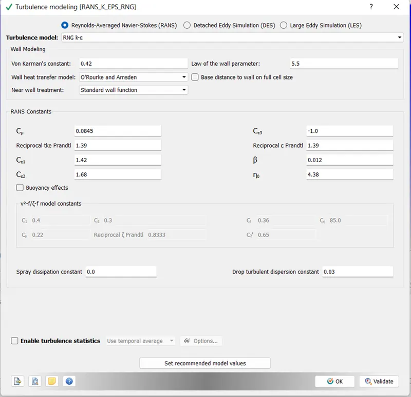
-Opt for Reynold’s Averaged Navier Stokes (RANS) RNG k-epsilon Turbulence model for the Turbulence Modelling.
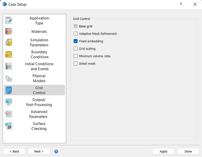
-To create refined mesh near the walls, opt for the Fixed embedding in the Grid Control tab.
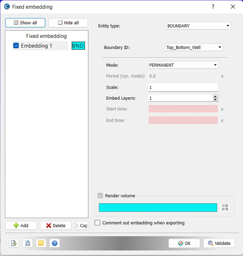
-Click on Add to create new Embedding. Select Boundary for the Entity type and Top_Bottom_Wall for the Boundary ID. Specify Scale and Embedded Layer as 1.
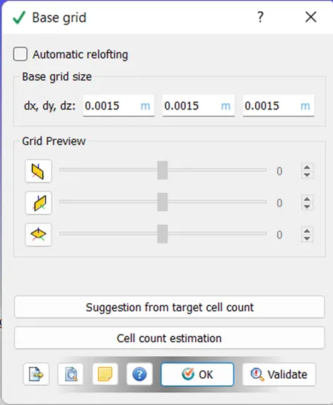
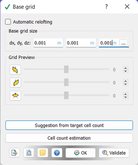
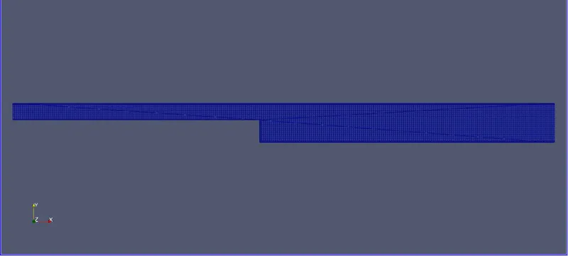
-Setup the mesh with 3 different grid sizes as mentioned below
dx = 2e-4m, dy = 2e-4m, dz = 2e-4m
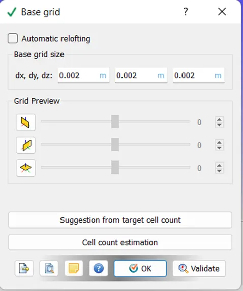
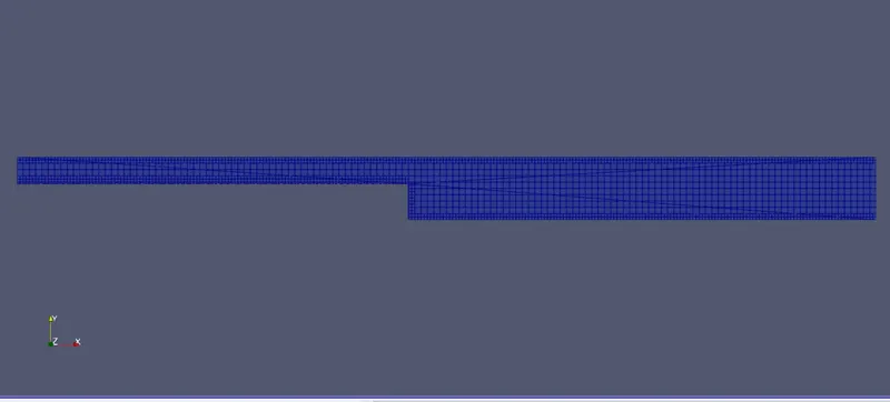
dx = 1.5e-4m, dy = 1.5e-4m, dz = 1.5e-4m
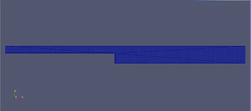
dx = 1.0e-4m, dy = 1.0e-4m, dz = 1.0e-4m
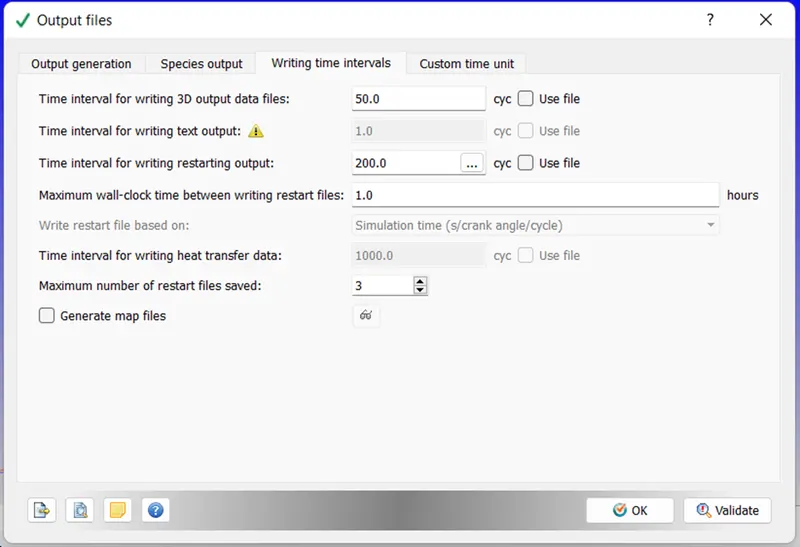
-In the Output file tab, specify the time interval for writing 3D output data files for 50 cycles. After 50 cycles it will create one 3D output file.
-The time interval for writing restarting output is specified as 200 cycles. If the simulation stops unexpectedly, it will help to restart the simulation in the last count of 200 cycles.
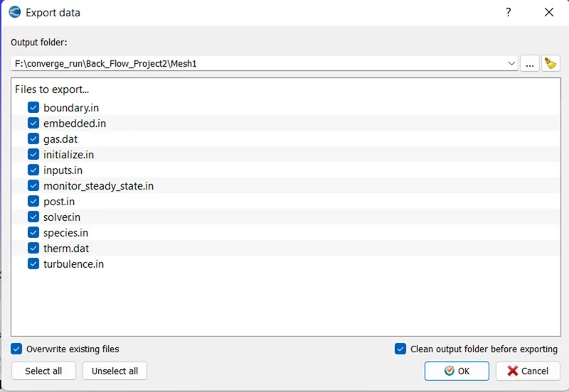
-After completing the simulation setup, export the input file to the desired folder. Click on the File then on Export. Select the Export Input Files option. Select the folder to export the input files and click on OK to complete the process.
Run the Simulation:
-To run the simulation, open the Cygwin terminal and open the folder which contains input files. Execute the command “mpiexec.exe -n 4 converge.exe restricted </dev/null> logfile &”. Before executing the command, paste the ‘mpiexec.exe’ and ‘converge.exe’ executables files into the input file’s folder.
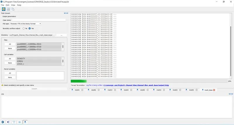
-On completion of the simulation, we need to convert the 3D output file which is readable for the Paraview.
-Open Post-Processing 3D in Converge Studio and specify the Case name. Select the Paraview VTK in-line binary Format for the File type. Select all the Post Files and Cell variables and click on Convert to complete the process.
Post-Processing:
-For post-processing, we will use the Paraview.
-Open Paraview and click on File to open the .vtm file from the Output folder. Click on OK
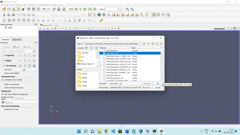
-Post-Processing is done in Paraview to obtain the plots and contours.
RESULT:
Case 1: Grid Size – 2e-4 m
Plots and Contours:
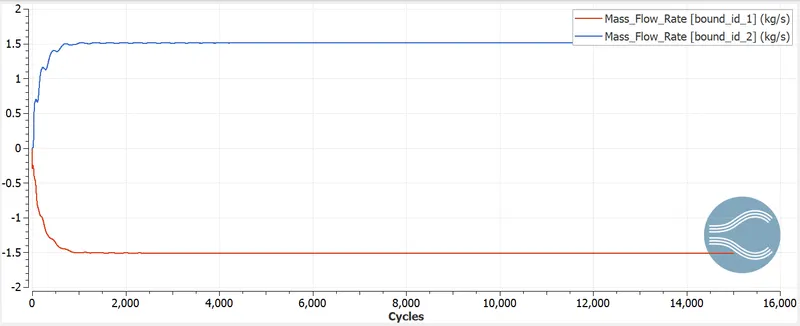
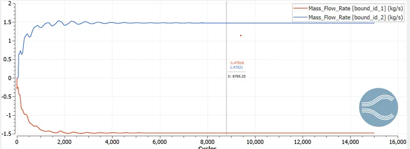
Mass Flow Rate vs Cycle (Inlet and Outlet):
Velocity:
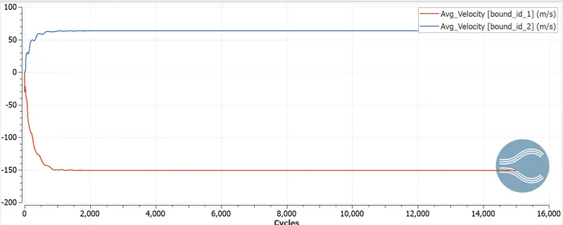
Velocity vs Cycle (Inlet and Outlet):
Velocity Contour:
Pressure:
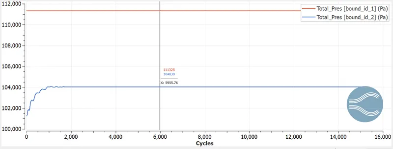
Pressure vs Cycle (Inlet and Outlet):
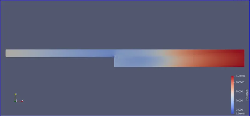
Pressure Contour:
Pressure Line Plot along X-axis:
Animation:
Velocity:
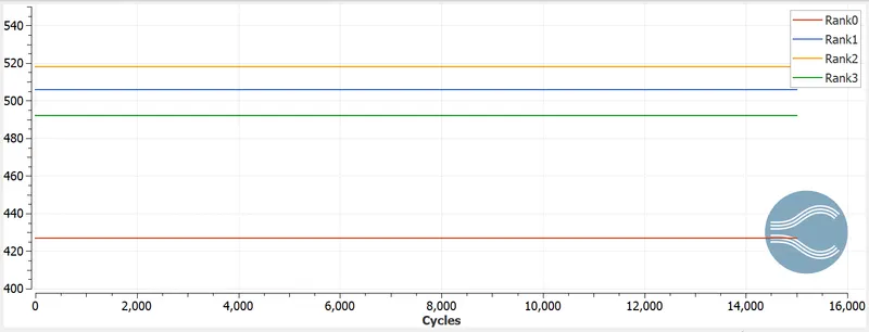
Total Cell Count:
Case 2: Grid Size – 1.5e-4 m
Plots and Contours:
Mass Flow Rate vs Cycle (Inlet and Outlet):
Velocity:
Velocity vs Cycle (Inlet and Outlet):
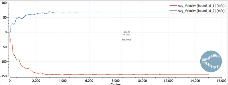
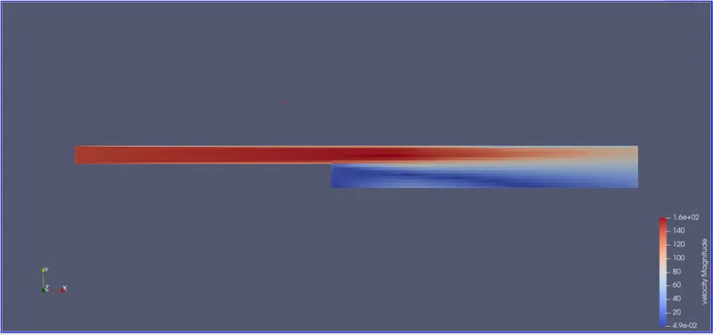
Velocity Contour:
Velocity Line Plot:
Pressure Plot:
Pressure vs Cycle (Inlet and Outlet):
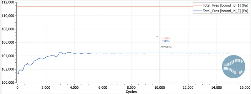
Pressure Contour:
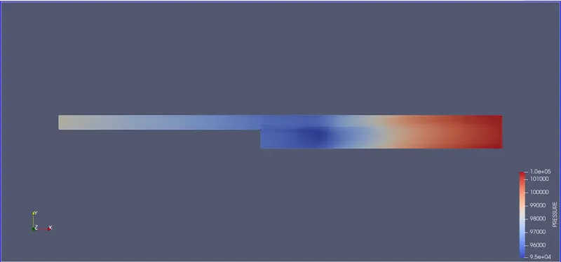
Animation:
Total Cell Count:
Case 3: Grid Size – 1e-4 m
Plots and Contours:
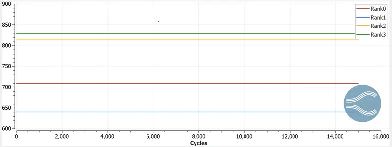
Mass Flow Rate vs Cycle (Inlet and Outlet):
Velocity Plot:
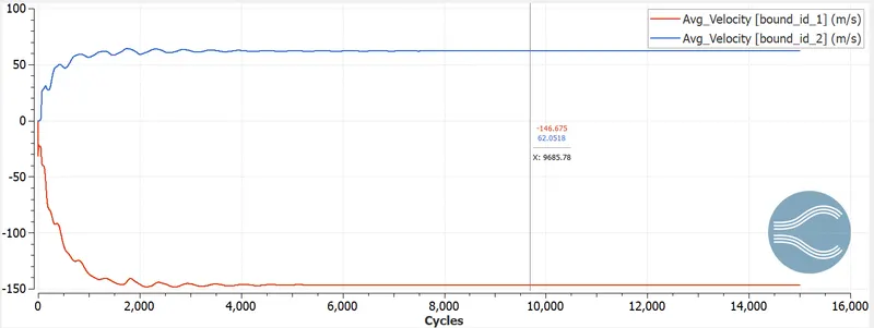
Velocity vs Cycle (Inlet and Outlet):
Velocity Contour:
Velocity Line Plot:
Pressure Plot:
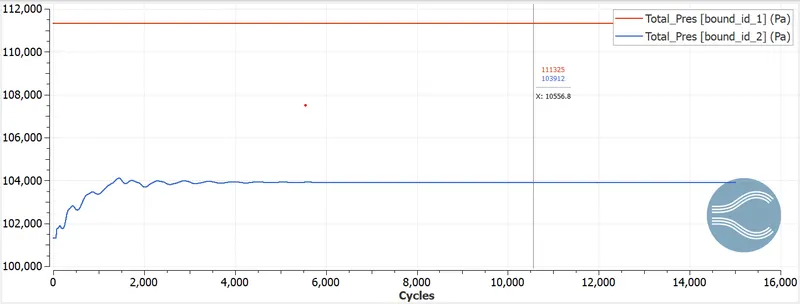
Pressure vs Cycle (Inlet and Outlet):
Pressure Contour:
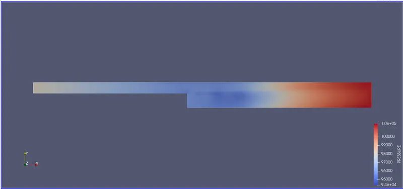
Animation:
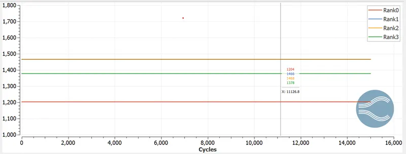
Total Cell Count:
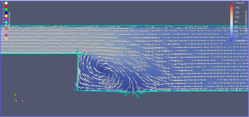
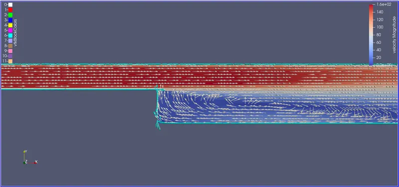
Vector Plot:
CONCLUSION:
- The flow over backward facing step is simulated using Converge CFD on 3 different meshes.
- The flow is conserved for all the 3 cases, which can be observed from the mass flow rate plot.
- In the vector plot, recirculation zone can be observe near the step. It is due to kinectic loss in the boundary layer region causes decreases in static pressure.