Week 7 - Simulation of a 1D Super-sonic nozzle flow simulation using Macormack Method
Simulation of 1-D Supersonic nozzle flow using Mac Cormack Method
In physics, different forms of governing equations does not have much significant difference as they all follows the same basic fundamental principle of fluid dynamics.
However in the world of Computational Fluid Dynamics, different form of governing equation leads to different results. One form of governing equation might give solution and other might results in oscillation or instability.
In this project, we will analyze the key difference in the conservative and non-conservative form of governing equation in terms of accuracy and stability by modelling and numerically solving 1-D quasi nozzle flow problem using Mac Cormack method.
Governing equation in Computational Fluid Dynamics
Governing equation in CFD also known as Naiver-Strokes Equation is the mathematical representation of the three fundamental principles of physics
- Mass is conserved.
- Rate of change in momentum is equation to force applied.(Newton’s second law)
- Energy is conserved.
Each principle is written in terms of equations and are known as Continuity equation, Momentum equation (Naiver-Strokes equation) and Energy equation respectively.
Conservative and Non-Conservative form of Governing equation
Conservative form of governing equation is the equation that is derived with the assumption of fixed fluid element whereas for Non-Conservative form, it is assumed that fluid element is moving in space.
Further these equation are classified based on their mathematical form as – Integral form and Differential form.
Non Dimensional governing equation in PDE form in
Non- Conservative form
1) Continuity equation - `(del rho')/(del t')= - rho' .(del V')/(del x') -rho'. V'.(del ln(A))/(del x') -V' (del rho')/(del x')`
2) Momentum Equation - `(del V')/(del t')= -V'.(del V')/(del x') -1/gamma.((del T')/(del x') + (T')/(rho' ). (del rho')/(del x'))`
3) Energy Equation - `(del T')/(del t') = -V'.(del T')/(del x') - (gamma -1).T'((del V')/(del x') +V'.(del ln(A')/(del x')))`
All the primitive variables are non dimesionalized
`x'=x/L` ; `rho'=rho/rho_o` ; `V'=V/a_o` ;`t'=t/(L/a_o)` ; `A'=A/(A^**)` ; `T'= T/T_o`
Where L is length of domain, `rho_0` is initial density value, `T_o` is initial temperature value `a_o` is speed of sound, `A^**` is throat area.
Conservative form
1) Continuity Equation - `(del(rho' A'))/(del t') + (del (rho' A'V'))/(del x') = 0`
2) Momentum Equation -`(del (rho' A' V'))/(del t') + (del(rho' A'( V')^2+(1/gamma).p'A') )/(del x') = (1/gamma).p'.(del A')/(del x')`
3) Energy Equation - `(del ( rho'A'*( (e')/(gamma-1) +(gamma/2). (V')^2)))/(del t) +(del ( rho'A'*( (e')/(gamma-1) +(gamma/2). (V')^2)+ rho'A'V'))/(del x') =0`
Since the above conservative form of governing equation is difficult to solve, these equations are simplified into a generic equation for 3-D flow.
`(del U )/(del t) +(del F)/(del x) +(del G)/(del y)+(del H)/(del z) = J`
where U is called solution vector; F,G,H are called flux vector and J is called source vector.
This equation is further simplified for 1-D flow
`U_1 =p'A'`
`U_2 = p'A'V'`
`U_3= rho'A'*( (e')/(gamma-1) +(gamma/2). (V')^2)`
`F_1 = p'A'V'`
`F_2 = p'A'(V')^2 +(1/gamma) p'A'`
`F_3 = rho'A'*( (e')/(gamma-1) +(gamma/2). (V')^2)+ rho'A'V'`
`J_2 = (1/gamma).p'.(del A')/(del x')``
With these term the governing equation become
Continuity equation - `(del U_1 )/ (del t') = -(del F_1)/ (del x' )`
Momentum equation - `(del U_2)/(del t') = - (del F_2 )/(del x' ) + J_2`
Energy equation - `(del U_3 )/(del t' ) = (del F_3 )/(del x' )`
Mac Cormack Method
The Mac Cormack method is an explicit finite difference technique consisting of two steps.
The initial step, known as the predictor step, involves discretization of the equations by implementing forward differencing to the spatial derivative terms in the RHS of the equation and solving the time marching equation.
Whereas in the second step, known as corrector step, spatial derivative terms are discretized by implementing backward differencing.
let us consider the continuity equation
`(del rho)/(del t)= - rho .(del V)/(del x) -rho. V.(del ln(A))/(del x) -V (del rho)/(del x)`
In predictor step, the continuity equation is discretized in forward differencing scheme
`((del rho)/(del t))_(i,p)^n= - rho .(( V _(i+1) -V_i)/(Delta x))^n -rho. V.( (ln(A_(i+1))- ln(A_i))/(Delta x) )^n-V (( rho_(i+1) - rho_i)/(Delta x))^n`
the predicted value for density`rho` for nth time step and i th node in the domain is
`rho_(i,p)^n = rho_i^(n-1) + ((del rho )/(del t ))_(i,p)^n **Delta t` (Taylor Series)
Value of `rho_(i,p)^n` is used in corrector step.
In corrector step, the continuity equation is discretized in backward differencing scheme
`(del rho)/(del t))_(i,c)^n= - rho .(( V _(i) -V_(i-1))/(Delta x))^n -rho. V.( (ln(A_(i))- ln(A_(i-1)))/(Delta x) )^n-V (( rho_(i) - rho_(i-1))/(Delta x))^n`
Again using Taylor series value of `rho`id determined
`rho_(i,c)^n = rho_i^(n-1) + ((del rho )/(del t ))_(i,c)^n **Delta t`
Now an average value of predictor and correction step is calculated
`rho_(i,avg)^n = 0.5**( rho_(i,p)^n + rho_(i,c)^n )`
This obtained value of `rho` is used for next time step and again all the above steps are iterated.
One Dimensional Quasi Supersonic Nozzle Simulation
A nozzle is a device which converts the pressure energy and thermal energy of the fluid into kinetic energy.
in a convergent-divergent nozzle (CD nozzle), the fluid enters into the nozzle in sub-sonic speed (M<1) and attains sonic speed at throat (M=1) and leaves the nozzle as exhaust gas at supersonic speed (M>1).
Nozzle shape is defined as
`A=1+2.2*(x-1.5)^2` where `0<=x<=3`
With initial condition
`rho = 1 - 0.3146**x`
`T = 1 - 0 .2314**x`
`V = (0.1 + 1.09**x)T^(1/2)`
Inlet Boundary Conditions is
`V_1 = 2**V_3 - V_2`
Oulet Boundary Conditions are
`rho_n = 2**rho_(n-1) - rho_(n-2)`
`V_n = 2**V_(n-1) - V_(n-2)`
`T_n = 2**T_(n-1) - T_(n-2)`
Main Program
Function for Non Conservative Form
%% *Function code to solve Non Conservative form of governing equation*

% Present MATLAB script is written as function to solve non-conservative
% form of governing equation using Mac Cormack method.

% Name of the Function is Non_Conservative.
% Which takes no. of grid point s in the domain (n), length of the domain or nozzle (l)
%   and  no. of time steps (nt).
% And as ouput it gives the distribution of density (rho_nc), velocity (v_nc),
% temperature (t_nc), mass flow rate (mf) , pressure (p_nc),
% Mach number (M_nc) inside the nozzle,
% time wise variation of mass flow rate ( mf_tnc ), density ( rho_tnc),
% velocity (v_tnc), temperature ( t_ tnc ) at throat for all time step
% and no. of time steps to attain steady state.


function [rho_nc,v_nc,t_nc,mf,p_nc,M_nc,mf_tnc,rho_tnc,v_tnc,t_tnc,k] = Non_Conservative(n,l,nt)


                  %% Defining  Domain

           n=31;              % No. of Grid points
           l=3;               % Length of the Nozzle (Domain)
           x=linspace(0,l,n);
           dx=x(2)-x(1);

                     %% Nozzle shape
         % Below equation defines Nozzle profile

            a=1+2.2*(x-1.5).^2;

                   %% Initial Conditions

    % Note:- All the varibles are in Non-Dimensional form

             g      = 1.4;                          % Adiabatic index
             rho_nc = 1 - 0.31468*x;                % Density
             t_nc   = 1 - 0.2314*x;                 % Temperature
             v_nc   = (0.1 + 1.09*x).* (t_nc.^0.5); % Velocity


                   %% Time step calculation

              c = 0.5 ;  % c=0.5 is assumed value for Courant number
                         %  as c must lies between 0 and 1

               nt =1400;  % No. of time step

               % Value for dt is obtain from CFL condition c = (dt/dx)*(a+v)
                % Where  a  is speed of sound

                       % It is assumed that   a = t^0.5
                                                                % dt at all grid points is calculated and
                   dt = min( c*( dx./ (t_nc.^0.5 + v_nc) ) );   % choose minimum value of dt


                      %% Mac Cormack method

           % Mac Cormack method is a two step process which involves Predictor and
           %  Corrector step for calulation

     for k=1:nt            % Begining of time loop

                 rho_old = rho_nc;
                   v_old = v_nc;
                   t_old = t_nc;
                      %%  Predictor step

           % In the Predictor Step, space derivative terms are discretized
           %  using Forward Differening.
           % And time derivative term is calculated
           %  to calculated predicted value of primitive variable using
           %    Taylor series


         for i=2:n-1                       % Begining of for loop for Predictor step


          % Forward Differentiation of space serivative terms
              drho_dx_f=(rho_nc(i+1)-rho_nc(i))/dx;
              dv_dx_f=(v_nc(i+1)-v_nc(i))/dx;
              dt_dx_f=(t_nc(i+1)-t_nc(i))/dx;
              da_dx_f=(log(a(i+1))-log(a(i)))/dx;

                 % Continuity Equation
    drho_dt_p(i)=-(rho_nc(i)*(dv_dx_f))-v_nc(i)*rho_nc(i)*da_dx_f-v_nc(i)*drho_dx_f;

                 % Momentum Equation
    dv_dt_p(i)=-v_nc(i)*dv_dx_f-(1/g)*(dt_dx_f+(t_nc(i)/rho_nc(i))*drho_dx_f);

                 % Energy Equation
    dt_dt_p(i)= -v_nc(i)*dt_dx_f-(g-1)*t_nc(i)*(dv_dx_f+v_nc(i)*da_dx_f);


                  %% Predicted value ( Primitive Varibles )

           rho_nc(i) = rho_old(i)+drho_dt_p(i)*dt;

             v_nc(i) = v_old(i)+dv_dt_p(i)*dt;

             t_nc(i) = t_old(i)+dt_dt_p(i)*dt;


             end              % Ending of Predictor Step


                   %% Corrector step

            % In the Corrector Step, space derivative terms are discretized
            %  using Backward Differening.
            %  And calculate the time derivative term
            %   using previously predicted primitive varible


                for i=2:n-1                  % Beginning of Corrector Step


                % Backward  Differentiation
            drho_dx_b=(rho_nc(i)-rho_nc(i-1))/dx;
            dv_dx_b=(v_nc(i)-v_nc(i-1))/dx;
            dt_dx_b=(t_nc(i)-t_nc(i-1))/dx;
            da_dx_b=(log(a(i))-log(a(i-1)))/dx;

                % Continuity Equation
       drho_dt_c(i)=-rho_nc(i)*dv_dx_b-v_nc(i)*rho_nc(i)*da_dx_b-v_nc(i)*drho_dx_b;

                % Momentum Equation
       dv_dt_c(i)=-v_nc(i)*dv_dx_b-(1/g)*(dt_dx_b+(t_nc(i)/rho_nc(i))*drho_dx_b);

                % Energy Equation
       dt_dt_c(i)= -v_nc(i)*dt_dx_b-(g-1)*t_nc(i)*(dv_dx_b+v_nc(i)*da_dx_b);


            end                % Ending of the Corrector Step


            %% Average of Predictor and Corrector Step


                % Average of time derivatives obtain from both
                %  the predictor and corrector step is calculated.
                % Average of time derivative terms are applied in
                %  the Taylor series to calculate primitive varibles
                %   Further obtained primitive variables are use for next time step as input

    for i=2:n-1


               drho_dt_avg(i) = 0.5*(drho_dt_p(i) + drho_dt_c(i));
               dv_dt_avg(i)   = 0.5*(dv_dt_p(i)   + dv_dt_c(i));
               dt_dt_avg(i)   = 0.5*(dt_dt_p(i)   + dt_dt_c(i));

             %% Calculating Primitive variable for next time step

               rho_nc(i) = rho_old(i) + drho_dt_avg(i)*dt;
               v_nc(i)   = v_old(i)   + dv_dt_avg(i)*dt;
               t_nc(i)   = t_old(i)   + dt_dt_avg(i)*dt;

    end


         %% Boundary condition

% Inlet Boundary Condition

% At inlet of the nozzle, we assume that only
% one of the primitive variable is floating
% i.e. velocity and the other two are fixed i.e. density and temperature.

             v_nc(1) = 2*v_nc(2) - v_nc(3);

% Outlet Boundary condition

% At outlet of the nozzle, we assume all the primitive variables are
% floating
            rho_nc(n) = 2*rho_nc(n-1) - rho_nc(n-2);
            v_nc(n)   = 2*v_nc(n-1)   - v_nc(n-2);
            t_nc(n)   = 2*t_nc(n-1)   - t_nc(n-2);

                         %%  Capturing time wise variation
         % Time wise variation of mass flow rate and primitive variables
         % at the Throat (n=16) are recorded and plotted against length of
         % the nozzle

      % Mass flow rate = rho * v * a;
         mf_tnc(k) = rho_nc(16)*v_nc(16)*a(16);

      % Density
         rho_tnc(k) = rho_nc(16);

      % Velocity
         v_tnc(k)  =  v_nc(16);

      % Temperature
         t_tnc(k)  = t_nc(16);

    %% Steady State

   % We assume that the system attains the Steady State if the absolute difference of one of the primitive variable i.e.
   % velocity in present and previous time step is less than 1e-5.
   % Time Loop is breaked and will stop further execution

 error = abs( v_old - v_nc );
   tol   = 1e-5 ;
   if error < tol
       fprintf(" System attains Steady State in %4.2f seconds ", dt*k)
       break
   end

     end                    % Ending of Time loop

       % Presure distribution inside the nozzle
       %  p = rho*t;
               p_nc  = rho_nc .* t_nc;

       % Mach number at each point of nozzle
       %  M is ratio of local velocity of fluid to the speed of sound

               M_nc  = v_nc ./ (t_nc.^0.5);
       % Mass flow rate at each point of nozzle.
       % Mass flow rate mf = rho * v * a

               mf = rho_nc .* v_nc .* a ;


end                          % Ending of the Function
Program for plots ( Non Consevative Form )
This program produces plot for steady state distribution of primitive varibles ( density, velocity, temperature) , time wise variation of primitive varibles and mass flow variation w.r.t time steps.
close all
clear all
clc

n= 31;
l=3;
x=linspace(0,l,n);
nt=1400;

%% Solution of Non-Conservative form of Governing equation
%   Using Mac Cormack method

[rho_nc,v_nc,t_nc,mf_nc,p_nc,M_nc,mf_tnc,rho_tnc,v_tnc,t_tnc,k]= Non_Conservative(n,l,nt);


%% Plot for Steady state primitive varibles w.r.t length of the nozzle

% Here Primitive varibles are velocity, density, temperature
figure(1)

% Plot Density vs Nozzle Length
subplot(3,2,1)
plot(x,rho_nc)
xlabel('Length of the Nozzle, x')
ylabel('\rho/\rho_o')
title('Density variation inside the Nozzle')
grid on

% Plot Mass Flow vs Nozzle Length
subplot(3,2,2)
plot(x,mf_nc)
xlabel('Length of the Nozzle, x')
ylabel('m/m_o')
title('Mass flow in the Nozzle')
grid on

% Plot Velocity vs Nozzle Length
subplot(3,2,3)
plot(x,v_nc)
xlabel('Length of the Nozzle, x')
ylabel('v/v_o')
title('Velocity inside the Nozzle')
grid on

% Plot Mach number vs Nozzle Length
subplot(3,2,4)
plot(x,M_nc)
xlabel('Length of the Nozzle, x')
ylabel('M')
title('Mach number')
grid on

% Plot Temperature vs Nozzle Length
subplot(3,2,5)
plot(x,t_nc)
xlabel('Length of the Nozzle, x')
ylabel('T/T_o')
title(' Temerature inside the Nozzle ')
grid on

% Plot Pressure vs Nozzle Length
subplot(3,2,6)
plot(x,p_nc)
xlabel('Length of the Nozzle, x')
ylabel('p/p_o')
title(' Pressure variation Inside the Nozzle ')
grid on


%% Plots for Time wise Variation
figure(2)
% Plot Mass flow rate vs Time Step
plot(1:k,mf_tnc)
title(' Variation in Normalized Mass Flow Rate at Throat w.r.t Time ' )
xlabel('Time Step')
ylabel('Mass Flow Rate ')

figure(3)

% Plot Density vs Time Step
subplot (3,1,1)
plot(1:k,rho_tnc)
title(' Variation in Density' )
xlabel('Time Step')
ylabel(' \rho/\rho_o')

% Plot Velocity vs Time Step
subplot(3,1,2)
plot(1:k,v_tnc)
title(' Variation in Velocity  ' )
xlabel('Time Step')
ylabel(' v/v_o')


% Plot Temperature vs Time Step
subplot(3,1,3)
plot(1:k,t_tnc)
title(' Variation in Temperature' )
xlabel('Time Step')
ylabel('T/T_o')
Function for Conservative Form
function [rho_con,v_con,t_con,mf_con,p_con,M_con,mf_tcon,rho_tcon,v_tcon,t_tcon,k] = Conservative(n,l,nt)

%                  %% Defining  Domain

           n=31;              % No. of Grid points
           l=3;               % Length of the Nozzle (Domain)
           x=linspace(0,l,n);
           dx=x(2)-x(1);

                     %% Nozzle shape
         % Below equation defines Nozzle profile

            a=1+2.2*(x-1.5).^2;

                   %% Initial Conditions

                % Adiabatic Index
                    g = 1.4;  % \gamma

                % Primitive variables
          % Density and Temperature
      %  Here, Density and temperature defination forms a profile
      %  from given initial condition

      for j = 1:n
          if ( x(j)>=0  &&  x(j)<=0.5 )
             rho_con(j) = 1;
               t_con(j) = 1;

                elseif ( x(j)>=0.5  &&  x(j)<=1.5 )
                   rho_con(j) = 1 - 0.366*(x(j) - 0.5);
                     t_con(j) = 1 - 0.167*(x(j) - 0.5);

                    elseif ( x(j)>=1.5  &&  x(j)<=3.5 )
                        rho_con(j) = 0.634 - 0.3879*(x(j) - 1.5);
                          t_con(j) = 0.833 - 0.3507*(x(j) - 1.5);

          end
      end

                   % Velocity
      % v = u_2*(rho*t) and
      % u_2 = rho*a*v; which represents mass flow rate

      % We assume that the mass flow rate throught the nozzle
      % is constant i.e. mass flow rate = u_2 = 0.59.

                    v_con = 0.59./(rho_con.*a);

   % Dependent variables/ Solution vector

                    u1 = rho_con .* a ;
                    u2 = rho_con.* a.* v_con;
                    u3 = rho_con.*a.*( (t_con./(g-1)) + ((g/2).*v_con.^2) ) ;

   % Time step value
                    nt = 1400 ;

       % Calculating dt using CFL Condition

          c  = 0.5;                                           % Courant Number
          dt = real( min( c*(dx./( (t_con.^2) + v_con ) )));  % dt

               %% Mac Cormack method

for k = 1:nt            % Beginning of Time Loop

        u1_old=u1;
        u2_old=u2;
        u3_old=u3;

         % Calculating Flux Vector
        f1 = u2;
        f2 = ((u2.^2)./u1) + (((g - 1)/g)*(u3 - ((g/2)*((u2.^2)./u1))));
        f3 = ((g*u2.*u3)./u1) - (g*(g-1)*(u2.^3))./(2*(u1.^2));

         %%  Predictor step
       for i= 2:n-1
           da_dx_p = ( a(i+1) - a(i) )/dx;
           J2 = rho_con(i)*t_con(i)*da_dx_p/g; % Source Vector

          du1_dt_p(i)= -( f1(i+1) - f1(i) )/dx;
          du2_dt_p(i)= -(( f2(i+1) - f2(i) )/dx) +J2;
          du3_dt_p(i)= -( f3(i+1) - f3(i) )/dx;

                 %% Predicted value

           u1(i) = u1_old(i) + du1_dt_p(i) *dt;
           u2(i) = u2_old(i) + du2_dt_p(i)*dt;
           u3(i) = u3_old(i) + du3_dt_p(i)*dt;
       end

             % Calculating flux vector for Corrector step
        f1 = u2;
        f2 = ((u2.^2)./u1) + (((g - 1)/g)*(u3 - ((g/2)*((u2.^2)./u1))));
        f3 = ((g*u2.*u3)./u1) - (g*(g-1)*(u2.^3))./(2*(u1.^2));

        rho_con = u1./ a;
        v_con  = u2./u1 ;
        t_con = (g - 1)*((u3./u1) - ((g/2)*(v_con.^2)));

             %% Corrector step
       for i=2:n-1
           da_dx_c = (a(i) - a(i-1))/dx;
           J2 = rho_con(i)*t_con(i)*da_dx_c/g;   % Source vector

          du1_dt_c(i)= -( f1(i) - f1(i-1) )/dx;
          du2_dt_c(i)= -(( f2(i) - f2(i-1) )/dx) +J2;
          du3_dt_c(i)= -( f3(i) - f3(i-1) )/dx;

       end

                %% Average of Predictor and Corrector Step
    for i=2:n-1


               du1_dt_avg(i)   = 0.5*(du1_dt_p(i) + du1_dt_c(i));
               du2_dt_avg(i)   = 0.5*(du2_dt_p(i)   + du2_dt_c(i));
               du3_dt_avg(i)   = 0.5*(du3_dt_p(i)   + du3_dt_c(i));

             %% Calculating Primitive variable for next time step

               u1(i)   = u1_old(i)   + du1_dt_avg(i)*dt;
               u2(i)   = u2_old(i)   + du2_dt_avg(i)*dt;
               u3(i)   = u3_old(i)   + du3_dt_avg(i)*dt;

    end
  %% Boundary condition

% Inlet Boundary Condition

        u2(1) = 2*u2(2) - u2(3);

 % Oulet Boundary Condition
       u1(n) = 2*u1(n-1) - u1(n-2);
       u2(n) = 2*u2(n-1) - u2(n-2);
       u3(n) = 2*u3(n-1) - u3(n-2);

        rho_con = u1./ a;
        v_con  = u2./u1 ;
        t_con = (g - 1)*((u3./u1) - ((g/2)*(v_con.^2)));
        %%  Capturing time wise variation
         % Time wise variation of mass flow rate and primitive variables
         % at the Throat (n=16) are recorded and plotted against length of
         % the nozzle

      % Mass flow rate = rho * v * a;
         mf_tcon(k) = rho_con(16)*v_con(16)*a(16);

      % Density
         rho_tcon(k) = rho_con(16);

      % Velocity
         v_tcon(k)  =  v_con(16);

      % Temperature
         t_tcon(k)  = t_con(16);

    %% Steady State
   % We assume that the system attains the Steady State if the absolute difference of one of the primitive variable i.e.
   % velocity in present and previous time step is less than 1e-5.
   % Time Loop is breaked and will stop further execution
 error = abs( u2_old - u2 );
   tol   = 1e-5 ;
   if error < tol
       fprintf(" System attains Steady State in %4.2f seconds ", dt*k)
       break
   end


end
       % Presure distribution inside the nozzle
       %  p = rho*t;
               p_con  = rho_con .* t_con;

       % Mach number at each point of nozzle
       %  M is ratio of local velocity of fluid to the speed of sound

               M_con  = v_con ./ (t_con.^0.5);
       % Mass flow rate at each point of nozzle.
       % Mass flow rate mf = rho * v * a

               mf_con = rho_con .* v_con .* a ;


end
Program for plots ( Conservative Form )
close all
clear all
clc

n= 31;
l=3;
x=linspace(0,l,n);
nt=1400;

%% Solution of Conservative form of Governing equation
%   Using Mac Cormack method

[rho_con,v_con,t_con,mf_con,p_con,M_con,mf_tcon,rho_tcon,v_tcon,t_tcon,k]= Conservative(n,l,nt);


%% Plot for Steady state primitive varibles w.r.t length of the nozzle

% Here Primitive varibles are velocity, density, temperature
figure(1)

% Plot Density vs Nozzle Length
subplot(3,2,1)
plot(x,rho_con)
xlabel('Length of the Nozzle, x')
ylabel('\rho/\rho_o')
title('Density variation inside the Nozzle')
grid on

% Plot Mass Flow vs Nozzle Length
subplot(3,2,2)
plot(x,mf_con)
xlabel('Length of the Nozzle, x')
ylabel('m/m_o')
title('Mass flow in the Nozzle')
grid on

% Plot Velocity vs Nozzle Length
subplot(3,2,3)
plot(x,v_con)
xlabel('Length of the Nozzle, x')
ylabel('v/v_o')
title('Velocity inside the Nozzle')
grid on

% Plot Mach number vs Nozzle Length
subplot(3,2,4)
plot(x,M_con)
xlabel('Length of the Nozzle, x')
ylabel('M')
title('Mach number')
grid on

% Plot Temperature vs Nozzle Length
subplot(3,2,5)
plot(x,t_con)
xlabel('Length of the Nozzle, x')
ylabel('T/T_o')
title(' Temerature inside the Nozzle ')
grid on

% Plot Pressure vs Nozzle Length
subplot(3,2,6)
plot(x,p_con)
xlabel('Length of the Nozzle, x')
ylabel('p/p_o')
title(' Pressure variation Inside the Nozzle ')
grid on


%% Plots for Time wise Variation
figure(2)
plot(1:k,mf_tcon)
title(' Variation in Normalized Mass Flow Rate at Throat w.r.t Time ' )
xlabel('Time Step')
ylabel('Mass Flow Rate ')

figure(3)
subplot (3,1,1)
plot(1:k,rho_tcon)
title(' Variation in Density' )
xlabel('Time Step')
ylabel(' \rho/\rho_o')
grid on

subplot(3,1,2)
plot(1:k,v_tcon)
title(' Variation in Velocity  ' )
xlabel('Time Step')
ylabel(' v/v_o')
grid on

subplot(3,1,3)
plot(1:k,t_tcon)
title(' Variation in Temperature' )
xlabel('Time Step')
ylabel('T/T_o')
grid on
Output / Result / Plots
Non-Conservative form
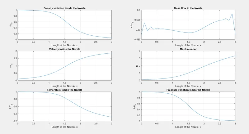
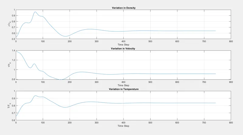
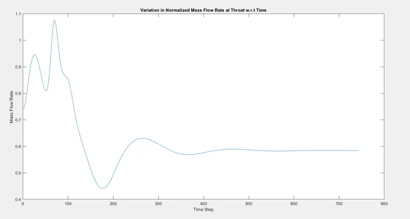
System attains Steady State in 14.96 seconds .
1. Plot showing steady state distribution of primitive variables inside the nozzle
2. Time-wise variation of the primitive variables
3. Variation of Mass flow rate distribution inside the nozzle at different time steps
Conservative Form
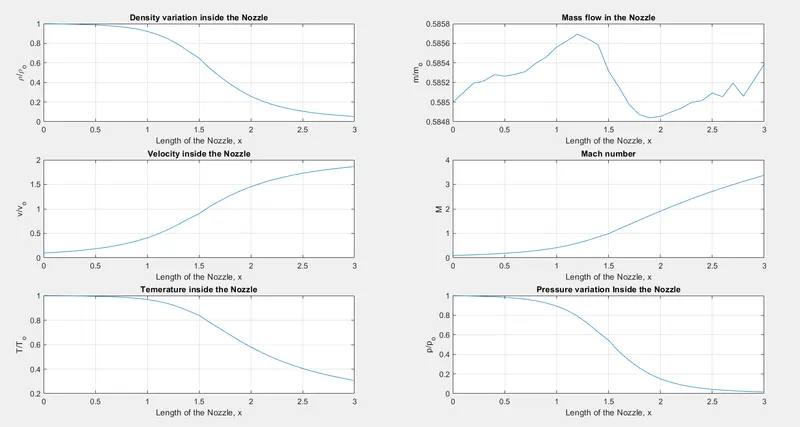
System attains Steady State in 14.26 seconds
1. Plot showing steady state distribution of primitive variables inside the nozzle
2. Time-wise variation of the primitive variables
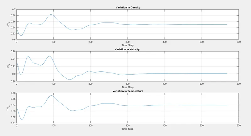
3. Variation of Mass flow rate distribution inside the nozzle at different time steps
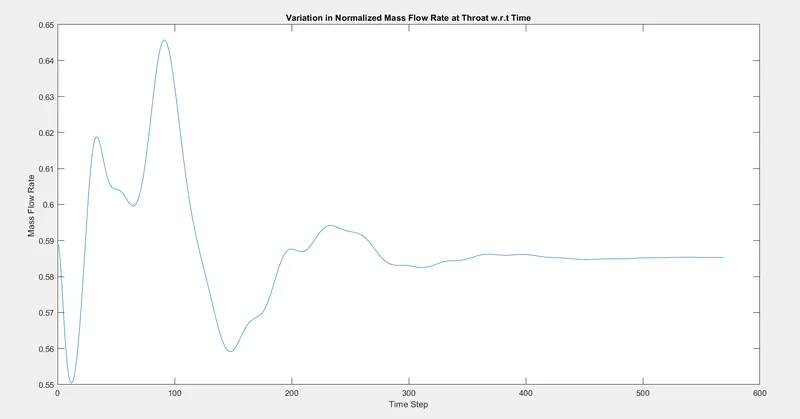
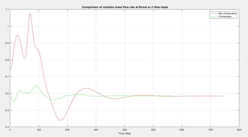
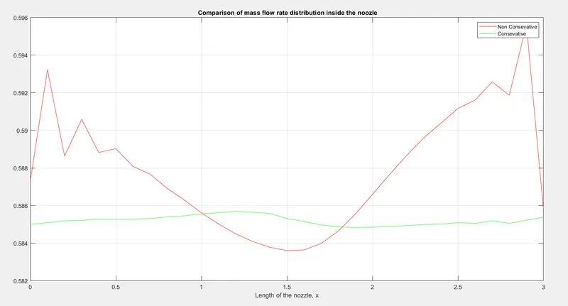
Comparison of Normalized mass flow rate distributions of Non-Conservative and Conservative form
Conclusion
1) From the result it is concluded that for the solution from both forms, system attains steady state nearly at same time.
2) There is no significant variation in the values of primitive variables calculated from both the form.
3) It can be observed that Conservative form converges more faster towards steady state than Non-Conservative form.
4) Solution from Conservative Form appears to be more stable than Non-Conservative Form.