Week 10: Project 1 - FULL HYDRO case set up (PFI)

AIM:
To perform simulation of Port Fuel Injection IC Engine.

OBJECTIVE :
To perform a full hydro simulation on a PFI IC engine and analyze the results.

DESCRIPTION :
In a PFI IC engine,fuel is injected prior to the valves and cylinder.The intake port will have a fuel injection system that sprays fuel into the air coming into the engine.From there spark plug ignite the pressurised slurry of air and fuel ,pushing the cylinder head down and spinning the crankshaft.

GIVEN DATA :

Engine Geometric Parameters

1. Bore =0.086 m
2. Stroke = 0.09 m
3. Connecting rod length = 0.18 m
4. RPM = 3000

Run parameters

1. Simulation mode: No Hydro

Simulation time parameters

1. Start time : -520 deg
2. end time : 120 deg

Boundary conditions

1. Piston temperature - 450K
2. Liner temperature - 450K
3. Head temperature - 450K
4. Spark Plug temperature - 550K
5. Spark Plug electrode temperature - 600K
6. Exhaust ports temperature - 500K
7. Exhaut outflow - 1 bar
8. Exhaust outlflow temperature - 800k
9. Exhaust species concentration - Calculate the stoichiometric condition
10. Exhaust valve top temperature - 525K
11. Exhaust valve angle temperature - 525K
12. Exhaust valve bottom temeprature - 525K
13. Intake port - 1 temperature 425K
14. Intake port - 2 temperature 425K
15. Inflow pressure - 1 bar total pressure
16. Inflow temperature - 363K
17. Inflow species - Air
18. Intake valve top temperature - 480K
19. Intake valve angle temperature - 480K
20. Intake valve bottom temeprature - 480K

Initial conditions

• Intake port - 1 (closer to combustion chamber)
  • ic8h18 - 0.025508
  • o2 - 0.20157
  • n2 - 0.77292
  • Temperature - 390k
  • pressure - 1 bar
• Intake port - 2 (away from combustion chamber)
  • Air
  • Temperature - 370K
  • Pressure - 1 bar
• Cylinder
  • Pressure - 1.85731 bar
  • Temperature - 1360K
  • Stoichiometric composition

Injection Parameters

1. Fuel flow rate = 7.5e-4 Kg/second
2. Injection start time = -480.0
3. Injection duration = 191.2
4. Fuel temperature = 330K

Nozzle positions

Nozzle diameter = 250 micro-meter

Circular injection radius = Nozzle radius

Spray cone angle = 10

• Nozzle 0
  • center 0.0823357 0.00100001 0.07019
  • Align Vector -0.732501 0.210489 -0.647408
• Nozzle 1
  • center 0.0823357 -0.00099999 0.07019
  • Align Vector -0.732501 -0.210489 -0.647408
• Nozzle 2
  • center 0.0823357 -0.0004 0.07019
  • Align Vector -0.5 -0.2 -0.647408
• Nozzle 3
  • center 0.0823357 0.0003 0.07019
  • Align Vector -0.5 0.2 -0.647408

Spark Ignition Parameters

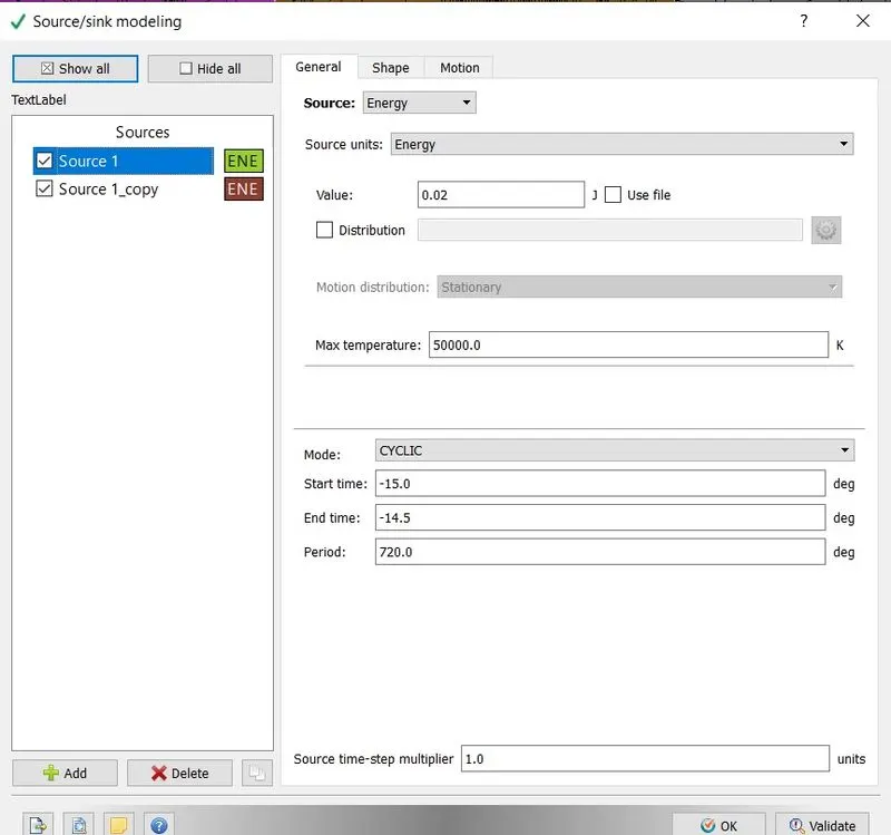
• Start of spark = -15 deg
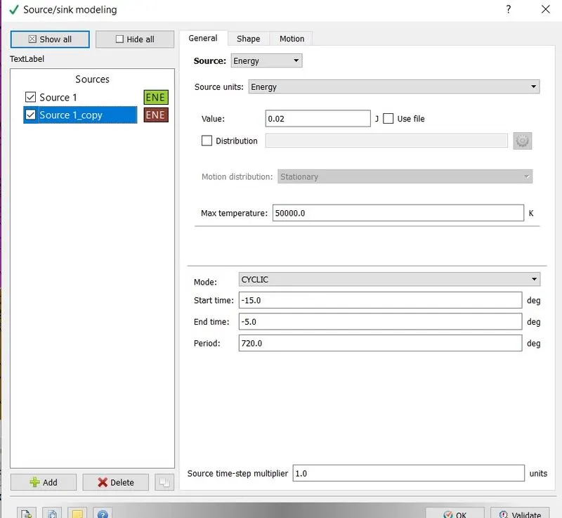
• Spark duration = 10 deg
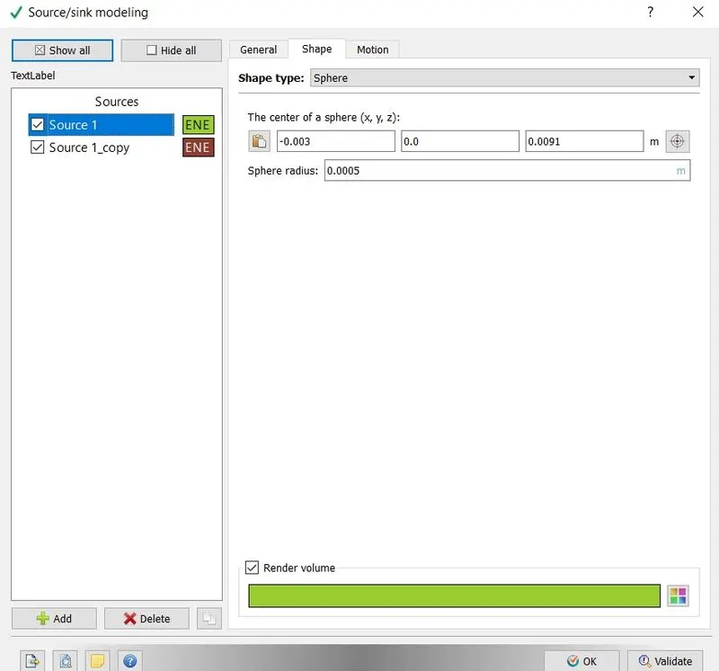
• Spark location = -0.003 0 0.0091
• Spark radius = 0.0005m

SOLUTION PROCEDURE :
To perform this simulation ,we will follow the below procedure :-

Case Setup --> Solution --> Post Processing

Case Setup :
Continuing from the previous project,change simulation mode to full hydrodynamic,

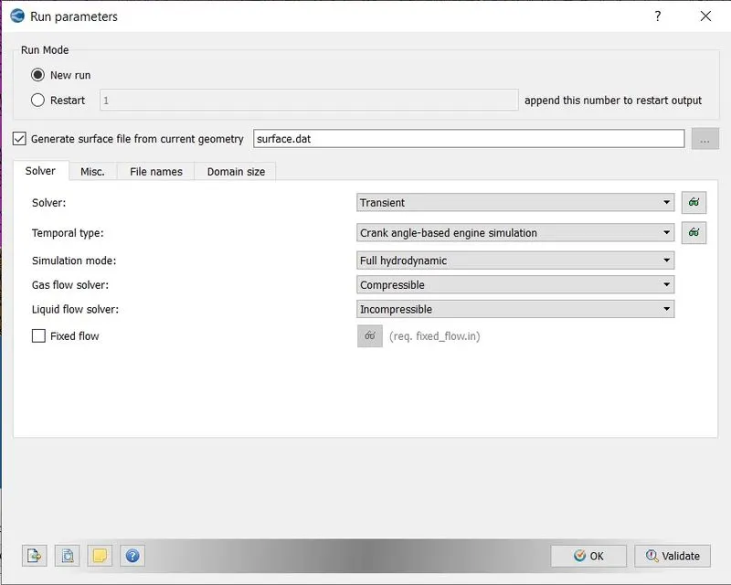
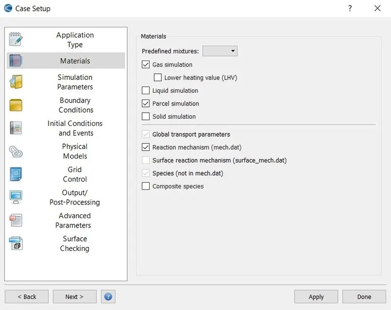
First,we need to tell converge which fuel we want to use for our simulation,
Go to materials => select Parcel simulation = Done.

Now we will define our fuel parcel,
Parcel Simulation => Predefined Liquids => select IC8H18_Isooctane => Add selected.

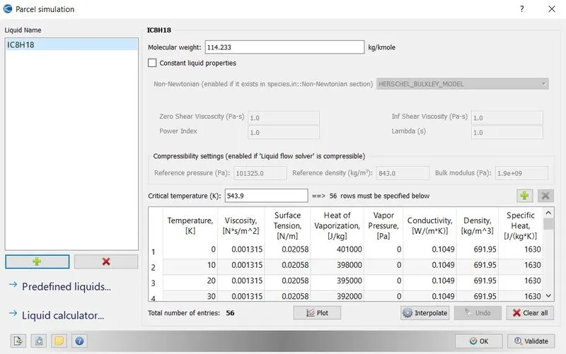
Here we are selecting iso-octane ,because it has properties very close to gasolene.If we were to use diesel fuel then we would have to select Diesel2.Physical properties of fuel used in experiments must match with the physical properties of parcel species we are using.

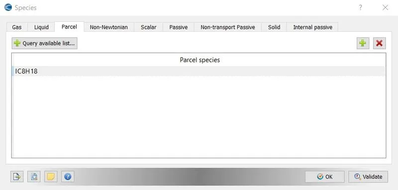
Species(we need to tell converge what are the participating species).We don't need to provide gasolene species because that is being taken care by reaction mechanism itself.But we need to specify parcel species.
Species => Parcel => click on Query available list => select IC8H18 => validate => ok.

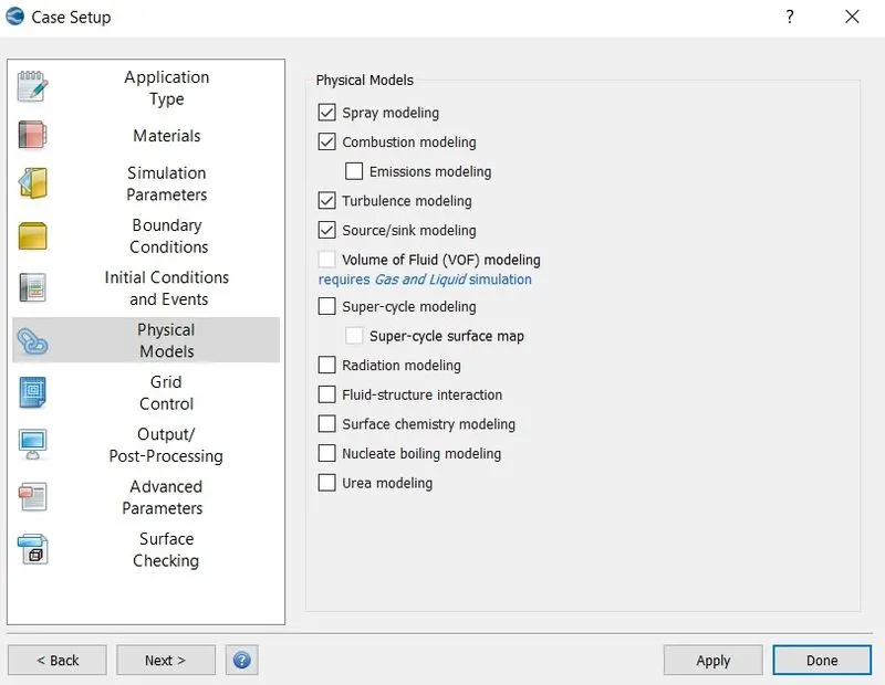
From physical models select spray modelling and combustion modelling.

SPRAY MODELLING :

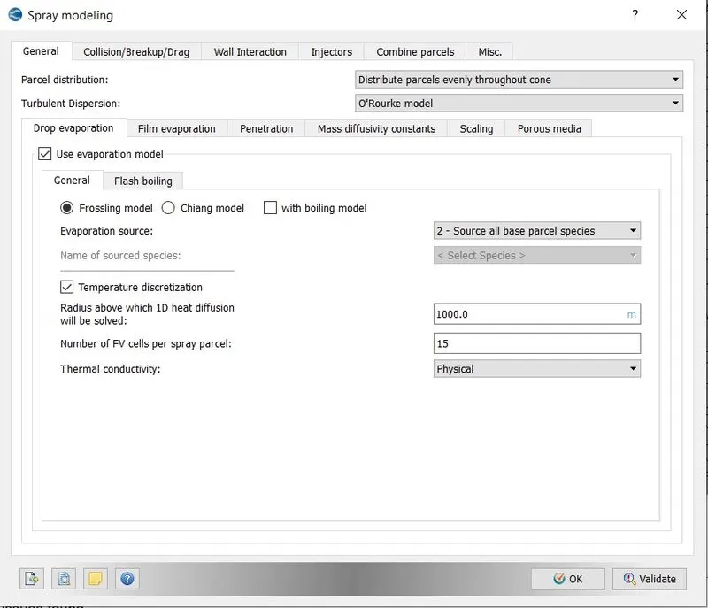
Unless specifically mentioned always select distribute parcels evenly throughout cone.As we have turbulence in our gas phase,these turbulence fluctuations are going to affect droplet characteristics.For gasolene sprays O'Rourke model has been shown to give better performance.We have selected frossling model Has evaporation model,which helps to dictate the rate at which our parcel radius is going to change.Source all base parcel species selected as evaporation source,this will convert liquid IC8H18 fuel into IC8H18 gas fuel.

Typically our fuel parcel is sphere.Outside of the sphere is hotter than the inside of the sphere.Typically a parcel is made up of drops that have only one temperature and there is no difference in the temperature.We can discretize the droplets by creating spherical finite volume cells.And solve the heat equation ODE on all of those individual finite volume cells. Although this process is more accurate ,it's time consuming.

When drop size is very very small,assuming that the entire drop is at the same temperature is more reasonable.And if drop is big,then there is going to be a gradient in temperature inside the drop.The maximum radius for ODE droplet heating is the cut off radius,above that radius ODE is solved and below that radius ODE isn't solved.Here we are putting larger value,that means
our ODE is never going to be solved and this will make our simulation run faster.Here we are sacrificing accureacy which is fine,because we don't have experimental data.

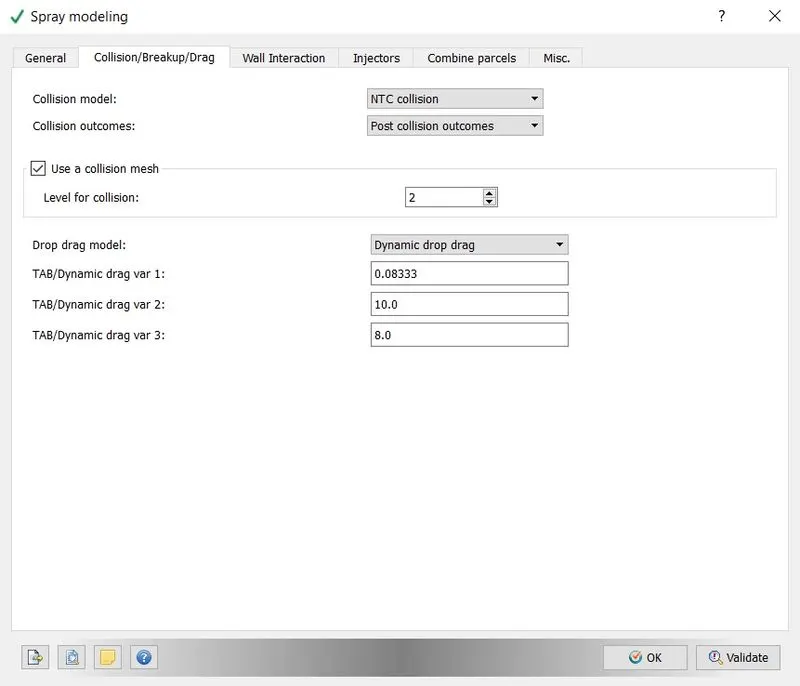
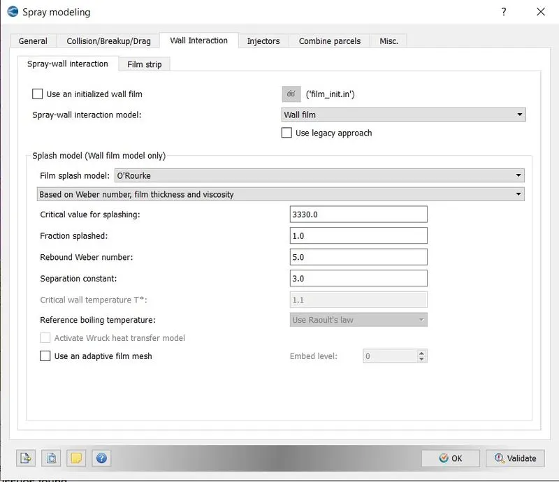
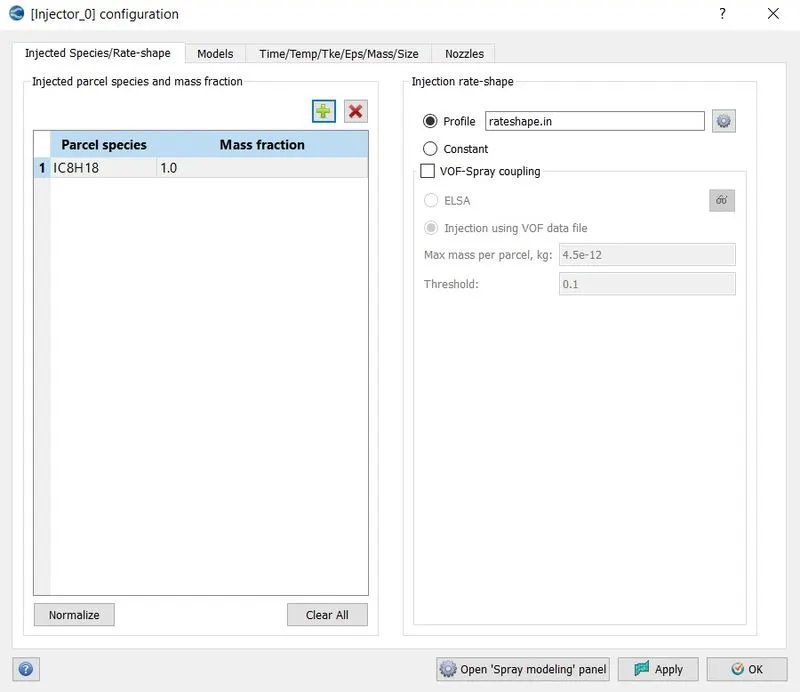
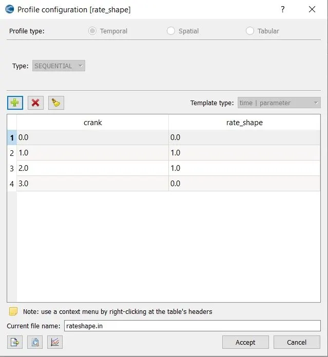
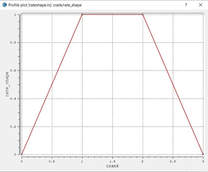
We used a collision mesh as this helps remove the grid effects in the final solution.Wall film has been selected as spray wall interaction model.When there is a wll film anu additional spary parcels can hit the wall film and it can splash.In the injected species we told converge what species are being injected.In injection rate shape converge will take the total mass of the
fluid that we have provided and the total duration that we have provided and it will use this profile to inject that mass accordingly within the time that we have specified.

COMBUSTION MODELLING :

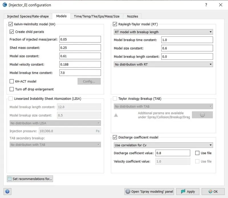
Kevin Helmhotz and Rayleigh Taylor,these are the models that are used for solid cone sprays ,it does not matter if it's diesel and gasolene.For traditional port fuel injector,tumble DI injector,DI diesel it's all going to be solid cone.

We can see there are some constants,these controls how our parcel is going to break up.There is an equation known as stability or dispersion equation which says how long it is going to take for disturbances on a perticular parcel to go unstable.With this equation we can come up with a logical time scale.But this equation is derived in a very simple manner,so we would have to put some constants so that we can increase or decrease the time it takes for the breakup to occur and also increase or decrease the size of the child.When Kevin Helmholtz model predicts the size of the child drop,we multiply the drop value by input value(here 0.6) which is mode size constant and reduce it.

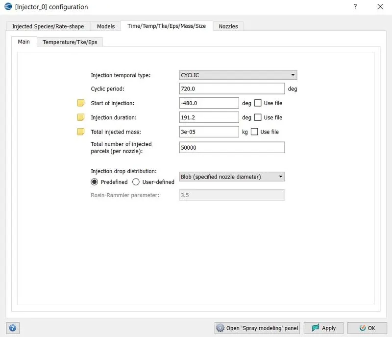
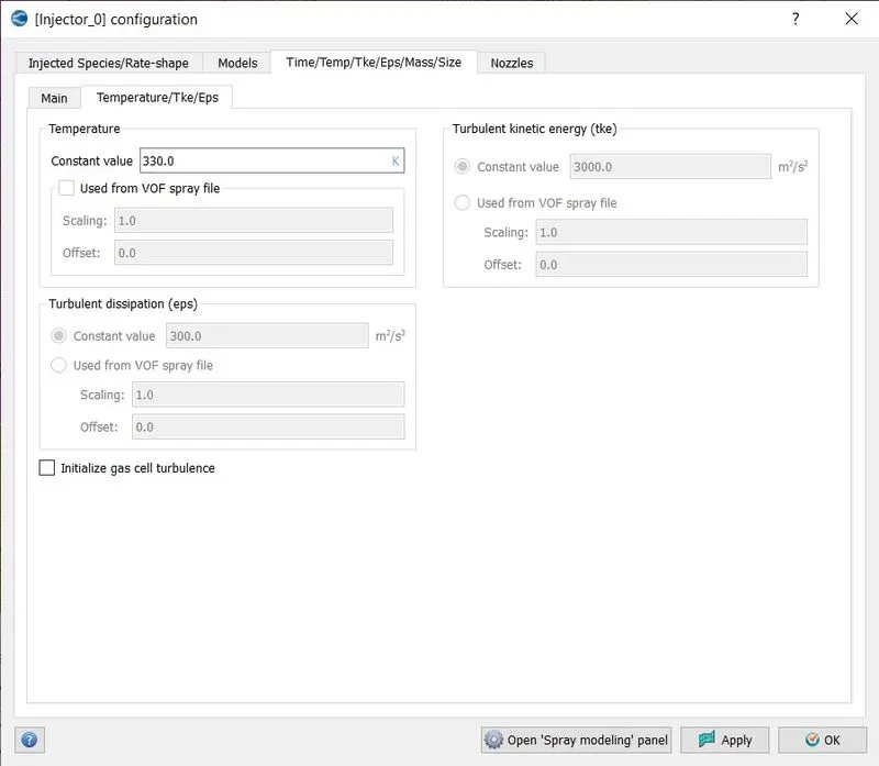
In the given data we have been given fuel flow rate in kg/sec.In engine fuel injection does not take place every second and it takes place for only some amount of time and then it stops. So having a single value of flow rate does not seem to make sense at the first place.But this flow rate can be converted into absolute mass.So in a 4 stroke engine,injection takes place at every 720 degrees.Hence for every 720 degrees there is a perticular value for time and for that perticular value of time we inject some amount of fuel.

RPM = 3000
Fuel Flow Rate = 7.5e-04
(Rounds Per Minute)RPS = 50
(Degrees per second)DPS = 18000
Time Per Degree = 5.5555 e-05
Time Per 720 Degrees = 0.04(Time Per Stroke)

As we know the flow rate in kg/sec,we can multiply these two quantities i.e. fuel flow rate and time per 720 degrees,we can get fuel mass per cycle which is,

Fuel Mass Per Cycle = 3e-05.

Nozzle Location And Orientation :

We can see that,we are getting injector at the center of the cylinder,but we want it in the intake port,to do that we will do the following steps,

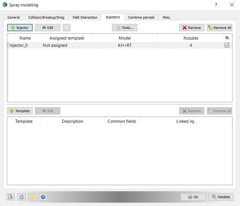
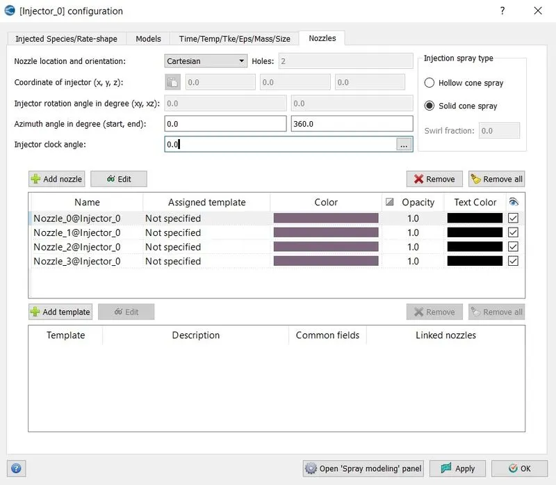
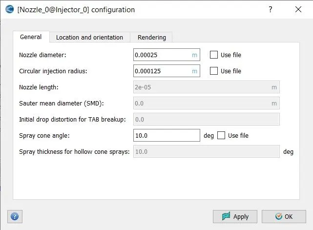
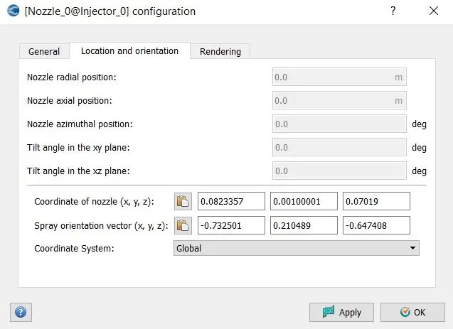
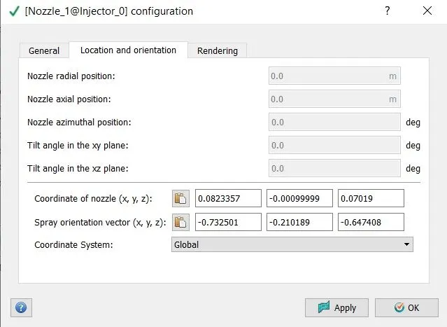
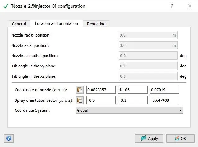
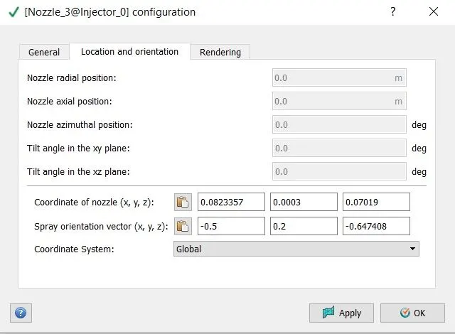
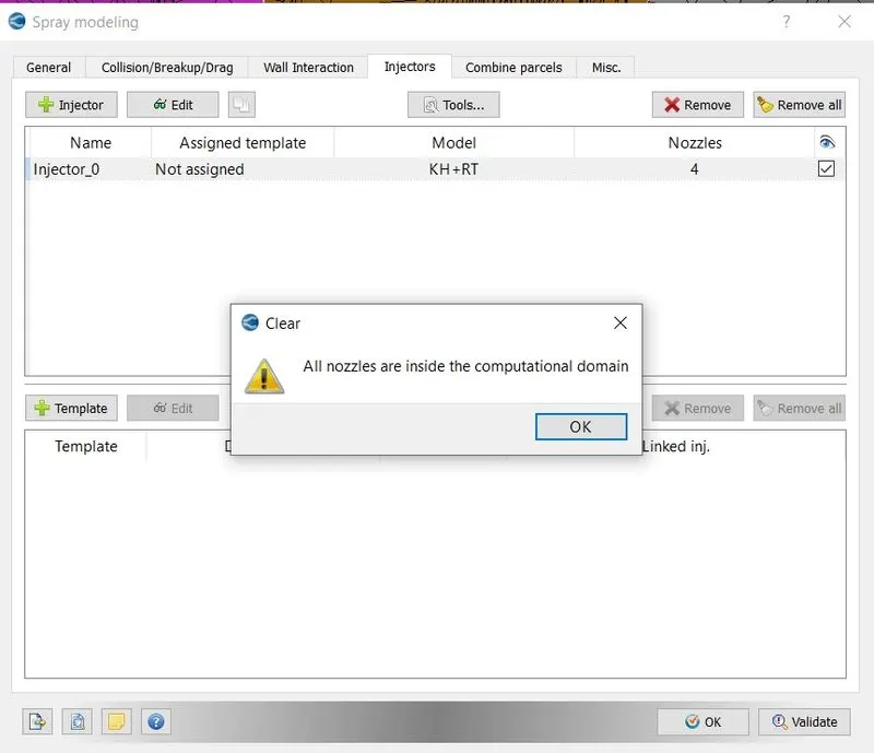
When we are specifying the nozzle,it can not be outside the geometry,hence follow the below steps,
spray modelling => Injectors => Tools => Validate Nozzle Locations => It should display the message as 'All nozzles are inside the computational domain'.

SAGE MODELLING :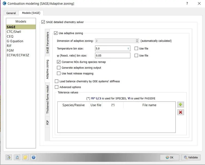

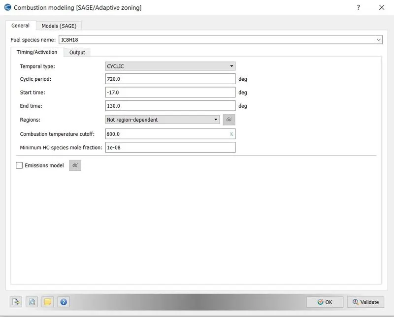
We used multizone model,this will speed up combustion calculations.Combustion should always start at few crank angles before the spark.Here we have choose -17degrees as combustion start time since,spark starts at -15 degrees.Combustion is going to end roughly when exhaust valve opens.Click on boundary,click on exhaust_lift.in file.From the file we can see that at around 120 degrees crank angle exhaust valve is opening,thus we have choose end time 130 degrees.

Spark Plug Setup :

Here our idea is that,we are going to introduce 2 energy sources,that are like spark plug.This energy is going to be sourced through energy equation and this is going to increase the temperature of the species and in species transport equation this temperature is going to be introduced.In species transport equation there is a source term,which is responsible for combustion to occur,that is going to see this temperature change and that is going to affect chemical kinetics,which is going to cause new product and subsequent hest release.Which is going to come back to the species equation,produce more species ,release more heat which is going to show up in energy equation which is going to increase the temperature.

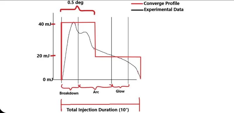
From the figure we can see that experimental spark data can be divided into 3 parts namely breakdown , ark and glow.During breakdown phase we putin more energy do that we are able to conduct through spark gap.Once we achieved breakdown phase we just need little bit of energy to keep the conduction going on.And it turns out that during the breakdown phase we provide 40 mJ of energy that lasts for a little bit and after that we provide 20 mJ.

In converge we reproducing above discussion by providing two energy sources.One energy source is going to lasts for 0.5 deg and will provide 40 mJ energy and another source will provide 20mJ and will last for 10 deg. Since both sources will be at same location at 0.5 deg so we will be dumping 40mJ of energy,thats why source one is at 0.02J cause 0.02J from source 2 will add in it.

FIXED EMBEDDING :

When we are this amount of energy(from above),we want to make sure that there is less numerical diffusion in those areas.So that we put the energy in and energy stays there long enough,so that it is able to combust the reactants.And for this we have to add additional refinement in that area,so we are going to add fixed embedding.

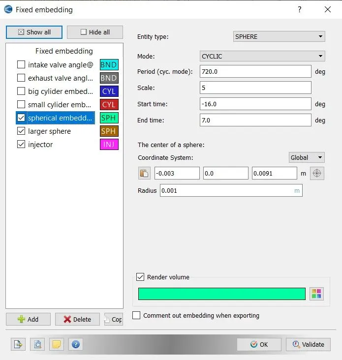
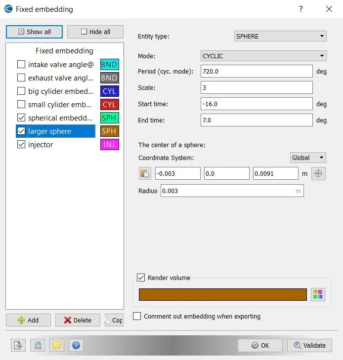
Here we have given start and end values such that,converge starts the emedding before spark and last 1 to 2 degrees after spark.

Why do we need this refinement ?

We will be using temperature AMR so that based upon curvature in the temperature field, cells will be refined.But when the spark is initially introduced ,just at that instant we don't have good refinement so that these gradience can be calculated accurately.So we are initially creating highly refined regions which lasts only for few crank angles,so that after some time,after
one or two time steps the temperature AMR is able to see that there is huge gradient or huge curvature change in temperature near the spark and then it's going to workout.
In other words this initial set of refinements is used to provide a better seed value for our AMR calculations.If the grid is very coarse the curvature values will also be low and AMR might not do anything about it.

AMR :

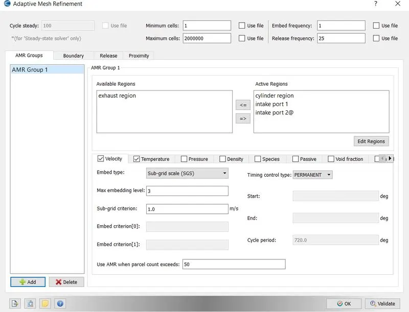
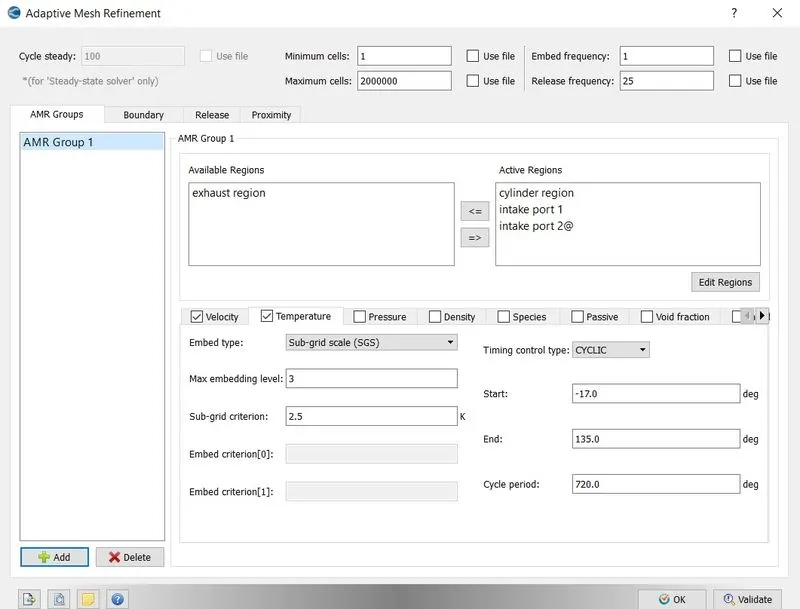
We set start time such that temperature AMR starts few crank angles before spark starts and ends when combustion ends.

INJECTOR EMBEDDING :

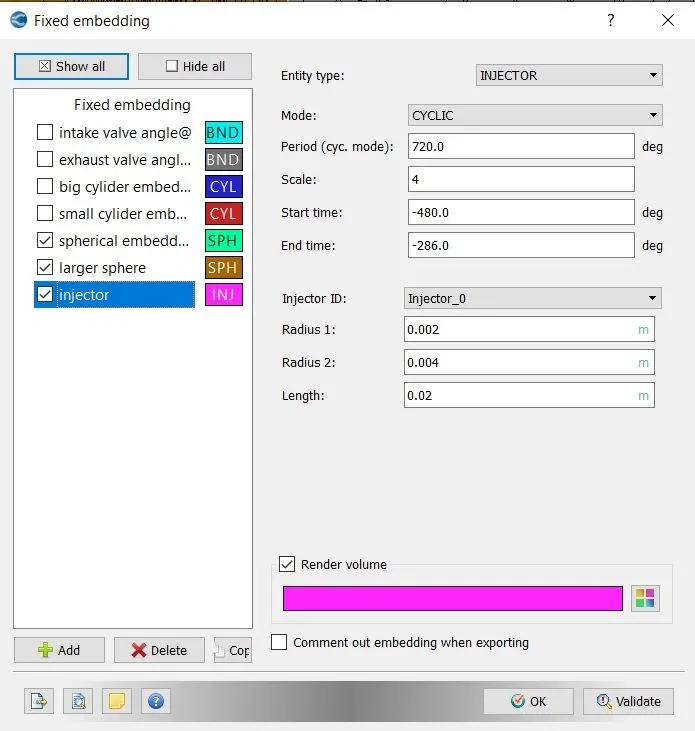
Our computational mesh size in injector region is 5 mm,so it is not going to calculate the second order derivative accurately,so we need to have initial refinement,so that we can calculate those derivatives accurately and then leave rest of the calculations to AMR,hence we are setting it up like this.

SOLUTION :

For running the simulation,first we need to export all the input files to the folder where we want to save our output files,

File => Export => Export Input Files => select the desired folder => Export.

Now we will use CYGWIN command prompt to run our simulation.But before running the simulation first we need executables
which willl solve the simulation,for that paste mpiexec.exe and converge.exe into the folder where we have exported all our input files.

Now using CYGWIN command prompt,navigate to the folder where all the input files are exported,and type the below command,

mpiexec.exe -n 4 converge.exe restricted </dev/null> logfile &

In the above command ,mpiexec.exe will help us to run our simulation in parallel,-n 4 are the number of cores on which we
want to run our simulation.As we are using the version of converge which has limit on the size of the file it can solve hence the command restricted.And the last part of the command dump all the data that is being generated into the logfile, which we can access during simulation procedure to see where our simulation has reached.

The above command will create a folder named output containing all the generated 3D output data.As we will be using paraview as the postprocessing tool.Hence we need to convert these output files into the format that paraview can read.For this we will use converge post convert tool.

Go to converge post processing 3D =>give case name => select the file type => navigate to the output folder and select it
=> select all files => select all variables => convert.

This will create group file ,which will be used by paraview to post process our results.

POST PROCESSING AND RESULTS :

The current case was setup with exhaust stroke beginning at first,followed by intake,compression and combustion.

Temperature Variation inside the cylinder -

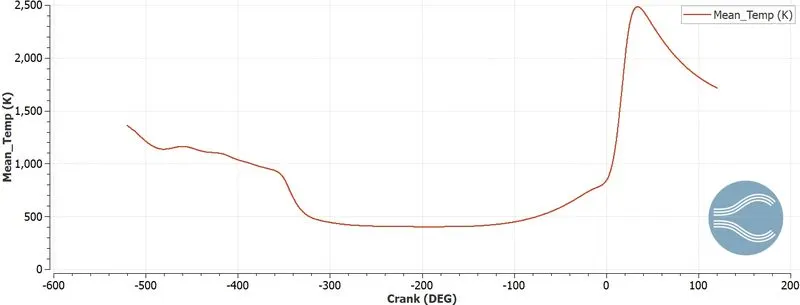
Since,the simulation is starting from exhaust stroke,a temperature rise can be seen at the start.After that there is temperature drop due to start of intake cycle,as cool air and fuel comes in.Then there is sudden temperature rise indicating start of expansion stroke and fuel combustion takes place and then exhaust stroke causing temperature drop.

Compression Ratio -

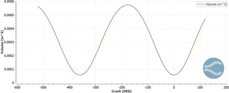
It is the ratio of the volume inside the cylinder when piston is at the bottom dead center to the volume when cylinder is at the top dead center.This is obtained by looking at the graph of volume inside the cylinder at different crank angles.

Maximumm Volume = `0.000574216 m^3`
Minimum Volume = `5.70298e-05 m^3`
Compresion Ratio = Max.Volume/Min.Volume = `0.000574216/0.0000570298`
Compresion Ratio = 10.07

Need of wall heat transfer model ?

The ability to predict heat transfer in engines plays an important role inengine development.Heat losses is the major limiting factor for the efficiency of the internal combustion engine.Furthermore,heat transfer phenomena causes thermally induced mechanical stresses compromising the reliabiltiy of engine components.
In CFD, thermal wall function models are used to calculate wall temperature.The assumptions made in the model leads to the model underpredicting wall heat losses as compared to experimental measurements.
The assumptions made in thermal wall function model includes :
1] Flow is parallel to the chamber walls with negligible flow normal to the walls.
2] Quasi Steady steady flow with negligible trsnsients.
3] Constant density and transport properties in the boundary layer.
4] High Reynolds number,very thin laminar shear layer.
5] Zero pressure gradients along the flow.
6] No combustion and chemically inert mixture

None of the above assumptions can be met with engines.The flow is neither one dimensional nor steady.Assumption three is perfectly invalid,because of large thermal geadients inside the boundary layer.Hence we need non equilibrium models to predict wall temperatures accurately.Some of the wall heat transfer models include Angelberger model,Werner Wengle model etc.

Why can't we predict the wall temperature from the CFD simulation ?

In IC engine to predict wall heat transfer we need to preform CHT analysis on engine cylinder.The CHT analysis allows the heat transfer between fluid and solid by exchanging thermal energy at the interface between them.In the current simulation we are not considering solid part and the simulation was only performed on the fluid domain.The Navier Stokes equations can predict
the temperature distribution across the fluid domain using the source term.Also CFD governing equations solves mass,energy and momentum equations related to compressible/incompressible fluids.But to model the heat transfer through the wall,a separate set of equations are required to predict the heat transfer through the solid such as conduction.thus with this setup we can't predict the wall temperatures.

Combustion Efficiency -

It is the ratio total heat released during the combustion to the total energy content of the fuel.Heat released is obtained from integrated heat rate plot.

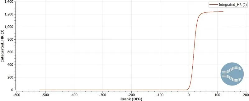
From the integrated heat released plot,the total heat released is 1241.1 J

`"Total heat content of the fuel" = "Amount of fuel per cycle" * "Calorific value"`

We know that,
RPM = 3000
Fuel Flow Rate = 7.5e-04
(Rounds Per second)RPS = 50
(Degrees per second)DPS = 18000
Time Per Degree = 5.5555 e-05
Time Per 720 Degrees = 0.04(Time Per Stroke)

As we know the flow rate in kg/sec,we can multiply these two quantities i.e. fuel flow rate and time per 720 degrees,we can get fuel mass per cycle which is,

Fuel Mass Per Cycle = 3e-05.

Calorific value of fuel = 44 MJ/kg
Total heat Content Of the fuel = `(0.00003*44*10^6) = 1320 J`

`"Combustion Efficiency, "eta_c = ("Total Heat Release")/("Total heat content Of fuel")`
`eta_c = (1241.1/1320)*100`
`eta_c = 94.0276 %`

Power and Torque -

Work = 468.646 N-m
Duration = 240.199 deg
RPM = 3000
(Rounds Per second)RPS = 50
Single rotation of piston = 360 Deg.
(Degrees per second)DPS = `360*50 = 18000`
Time taken be the piston for complete rotation = `240.199/18000 = 0.01334 sec`
`"Power" = "Work Done"/"Time Taken"`
=`468.646/0.01334`
P = 35130.885 W

Torque :

`P = (2*pi*N*T)/60`
`T = (P*60)/(2*pi*N)`
`T = (35130.885*60)/(2*pi*3000)`
T = 111.88 Nm

Significance of CA10,CA50 and CA90 -

CA10 - It is the crank angle at which 10% of the fuel has been burnt or the heat rate is 10% of cumulative HR.It's value is 6.83717 deg.

CA50 - It is the crank angle at which 50% of the fuel has been burnt or the heat rate is 50% of cumulative HR.It's value is 18.4623 deg.

CA90 - It is the crank angle at which 90% of the fuel has been burnt or the heat rate is 90% of cumulative HR.It's value is 31.701 deg.

Pressure Variation With Crank Angle -

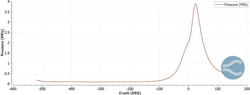
Pressure variation inside the cylinder is in tune with temperature plot.Slight high pressure at the start of the simulation,then drop during intake stroke and sudden increase during compression stroke and again reduction due to exhaust stroke.

Change in Mass With Crank Angle -

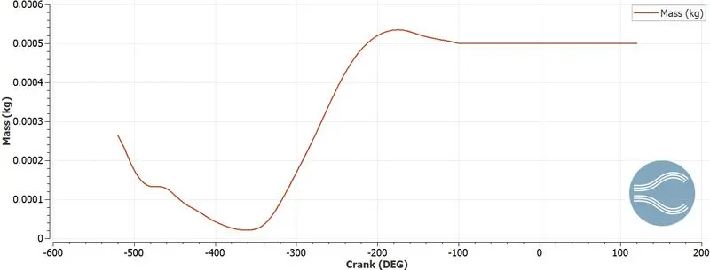
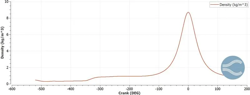
Density Variation With The Crank Angle -

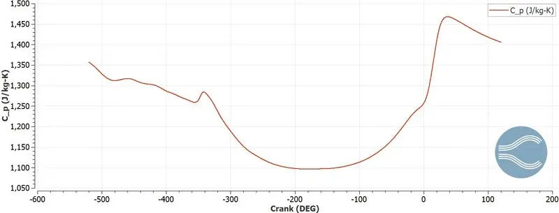
Cp Variation With The Crank Angle -

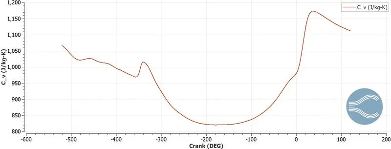
Cv Variation With The Crank Angle -

Gamma Variation With The Crank Angle -

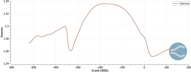
In theoretical calculations,we consider the constant value for gamma as 1.4.But it changes as a function of crank angle.

Liquid Spray Drops in The Cylinder -

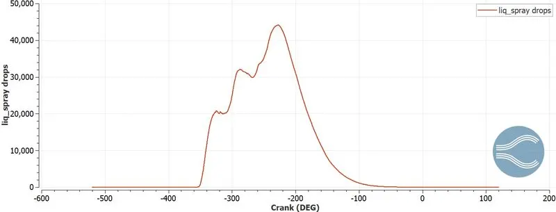
Using this plot we can evaluate the Lagrangian parcels that are active in the domain.At the end of the combustion there is no fuel left in the cylinder,means complete combustion had been taken place.

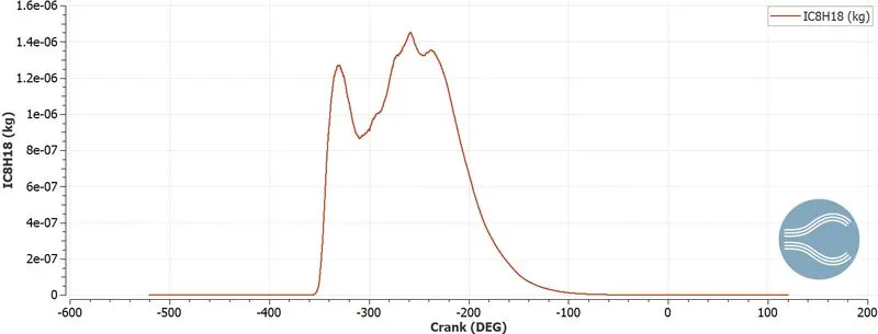
The Amount of Fuel Variation in Cylinder With The Crank Angle -

Liquid Sprey Drops Variation in Intake Port -

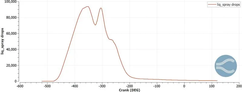
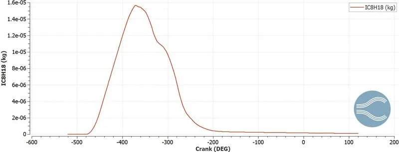
Some amount of fuel stays present inside intake port.
Emission Plots -

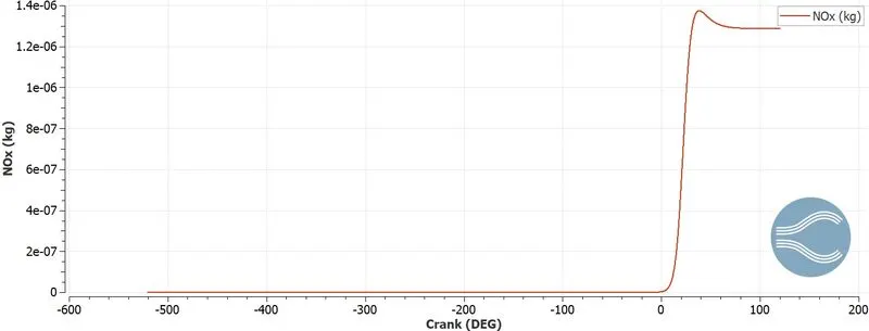
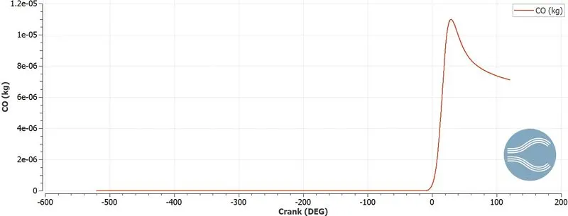
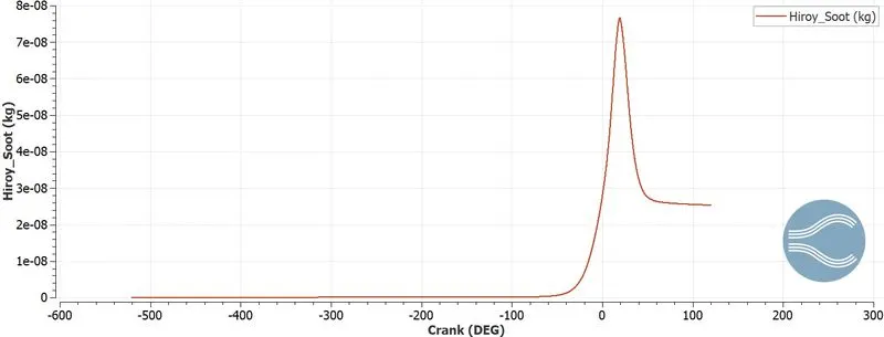
From the above plots we can that emissions are formed in exhaust and cylinder region.In the above plots we can see that Nox and Soot levels are minimal which indicates that combustion is almost complete leading to a small amount of unburnt of HC.

Animations -

Spray : https://www.youtube.com/watch?v=FycdsfSLVHU

Pressure : https://www.youtube.com/watch?v=XFIFiSj_L2w

Spray Parcel Temperature : https://www.youtube.com/watch?v=TT7Q8s4C0y4

Mass Fraction of IC8H18 : https://www.youtube.com/watch?v=PloC2QEwy3U

Conclusion -

The Full Hydro simulation of a PFI engine has been successfully performed using RANS k-epsilon model,coarser grids and larger time steps,which provdes approximated results but saves a lot of computational time and power.