Week 9 - Parametric study on Gate valve.

1].Aim -

To perform a parametric study on a gate valve.

2].Objective -

*To perform parametric study on the gate valve simulation by setting the opening from 10 % to 80 %
*Obtain mass flow rate at outlet for each opening.
*Calculate flow coefficient and flow cofactor for each opening.
*Plot graphs of flow coefficient vs lift and flow factor vs lift.
*Discuss the results of the mass flow rate and flow coefficient for increasing lift.

3].Introduction and Theory -

A gate valve, also known as a sluice valve, is a valve that opens by lifting a barrier (gate) out of the path of the fluid. Gate valves require very little space along the pipe axis and hardly restrict the flow of fluid when the gate is fully opened.

Gate valves are used to shut off the flow of liquids rather than for flow regulation. When fully open, the typical gate valve has no obstruction in the flow path, resulting in very low flow resistance.The size of the open flow path generally varies in a nonlinear manner as the gate is moved. This means that the flow rate does not change evenly with stem travel. Depending on the construction, a partially open gate can vibrate from the fluid flow.

When flow goes through a valve or any other restricting device it loses some energy.The flow coefficient is a designing factor which relates head drop(`Deltah`) or pressure drop (`DeltaP`) across the valve with the flow rate(Q).Each valve has it's own
flow coefficient.This depends on,how the valve has been designed to let the flow going through the valve.Therefore the main difference between different flow coefficients come from the valve,and opening position of the valve.

Flow coefficient is important in order to select the best valve for specific application.If the valve is going to be open most of the time,so the valve with less head loss would be the better choice.Or if it is needed a control valve,the range of coefficients for the different opening positions of the valve should fit the requirements of the application.

`K_v` is the flow coefficient in metric units.It is defined as the flow rate in cubic meters per hour(`m^3/h`) of water at a
temperature of `16^circ`C with the pressure drop across the valve of 1 bar.
`C_v` is the flow coefficient in imperical units.It is defined as the flow rate in US gallons per minute(gpm) of water at a
temperature of `60^circ` Fahrenheit with a pressure drop across the valve of 1 psi.

`K = Q*sqrt(S_g/(Deltap)`

where, Q -rate of flow
`S_g` - specific gravity of the fluid
`Deltap` -pressure drop across the valve

K = `C_v` ,when K is referenced in (gpm) (psi) units.
K = `K_v` ,when K is referenced in (m^3/h) (bar) units.

Relation between`K_v & C_v`

`K_v = 0.865*C_v`

`C_v = 1.156*K_v`

4].Methodology -

First we have to activate parameters at appropriate points throughout the simulation in order to get desired output.Then we have to make sure that fluid volume is adapted to the changing solid geometry.

5].Solution Procedure -

To simulate Gate Valve ,we will follow the below procedure :-

Geometry Creation --> Meshing --> Setup --> Solution & Post Processing

5.1].Geometry Creation -

* Launch the Ansys workbench.First drag and drop the Fluid Flow(Fluent)model into project schematic and double click on geometry to launch the SpaceClaim.
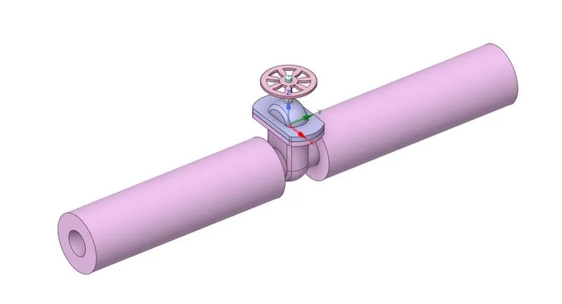
* Import the geometry into the ansys spaceclaim.Below we can see the image of the 3D view of the gate valve model used in
this project.

                                       
*First pull both outer surfaces(inlet and outlet) by 800 mm using pull tool in design tab.
*Now to extract fluid volume,
click Prepare => volume extract => select edge selection => select all inlet & outlet edges and top edge of bottom => ok.

                                      
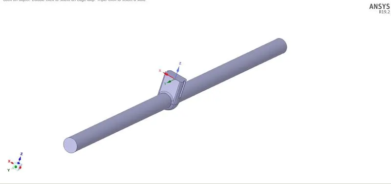
*Hide and supress all solid bodies.
*Now to parametrize the valve lift follow the below procedure-
1)in Design => select move and select gate disc and move it little bit up.
2)If we go to groups window(beside structure window),we can see that create parameter button has been activated,click on it and we will see Group 1 appear,in which we can edit the dimensions of the lift.

                                                    
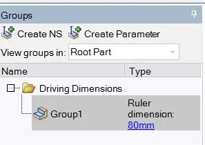
3)Update the extracted volume and update it as per the context,so that the fluid volume will adapt automatically to the lift.
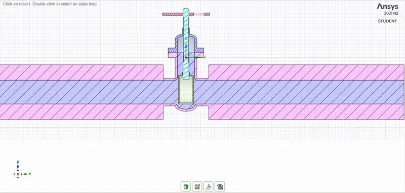
Make sure that spindle is visible.
*Below is the section view with 10 mm valve lift.

                                 
*close SpaceClaim.

5.2].Meshing -

*Now,go to meshing, by double clicking on mesh,and first do the name selection i.e give proper boundary names.Then generate the basic mesh using generate mesh command.We can see the flow of the mesh inside the extracted volume by using section plane.Also we can check the mesh quality by using mesh quality option.

select the prefered body => press N => name the selection.

In meshing we can see the mesh is perfect.Always create the named selection first before generating the mesh.Select the edge you want to name,click N & name the selection.This way create named selection for inlet & both outlets.

*Then,next thing to do is to mesh.We click the mesh option in the side window and create our base line mesh.We then refine
mesh by giving element size as 6 mm.
*Below is the geometry with final mesh.

                                    
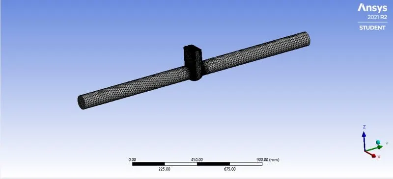
* Now lets check our mesh quality.Our minimum mesh quality is good enough.
* This concludes our meshing procedure.
* Now close the mesh & update.

5.3].Setup -

* Double click setup in project schematic.This will open ansys fluent.
*Click on check mesh and make sure there are no errors.

5.3.1] Setting up Physics
*Our solution method will be SIMPLE.

5.3.2] General -
*Solver type - pressure based
*time - Steady state
*velocity formulation - absolute
* We need to enable gravity.Since our geometry is in YZ-plane,give negative value for acceleration due to gravity.
General => Gravity =>Gravitational acceleration => Z(m/s) = -9.81 m/s.

5.3.3] Models -
*viscous model - k-epsilon Realizable with scalable wall functions.

5.3.4] Material -
*Fluid - Water-liquid

5.3.5] Zones -
Cell zone - In cell zone we can see our fluid volume ,Set it to fluid type,with material air change it to water.

5.3.6] Boundary conditions - We can see all the named selections which,we generated above being used as boundary conditions.

* Inlet -
Type - Pressure inlet
Total Gauge Pressure- 10 Pa

* Outlet -
Type - pressure outlet
gauge pressure - 0 Pa

*Now initialize the domain.We will use hybrid initialization,this provides very good initial conditions.
*We want to moniter different flow quantities as the solution is being generated,will use contours for this.We want to see how
the velocity and pressure & mass flow rate looks like.

*To create mass flow rate plot,
in definitions => flux report => mass flow rate => select outlet boundaries =>check report file and report plot => at the bottom select/mark the output parameter.

*To see contour plots,let's first create a plane.
postProcessing => create => plane => select YZ plane & hit create.

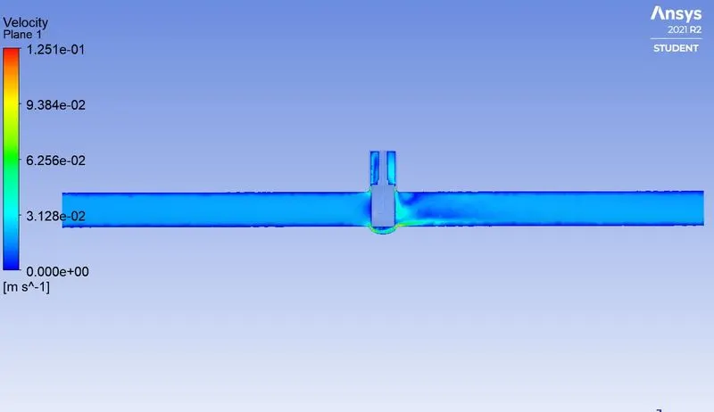
For velocity contour go to postProcessing => contours => new => contour of => velocity => under it velocity magnitude=> select plane & hit save/display.Simillarly create contour for pressure.
*To create animation,go to activities => solution animation => select velocity contour => preview => set desired view => give name
as velocity animation.

5.3.7] Solving -
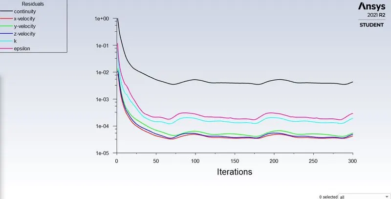
* We will run the simulation for 300 iterations.We can see from the residual plot that our solution has converged and reached the steady state.

5.4] Post Processing -

Residual Plot -
*It can be observed from the residual plot that solution has converged.

                                    

Mass Flow Rate Plot -
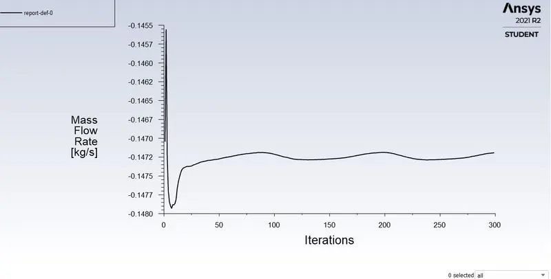
*We can see from the below plot,we are getting a good conserved value for mass flow rate.From the console we can see that
mass flow rate value is `-0.147190` `(kg)/s`.The negaive sign indicates that mass flow is leaving the domain,which validates that our solution setup is correct.

                                 

Velocity Contour -

                                   
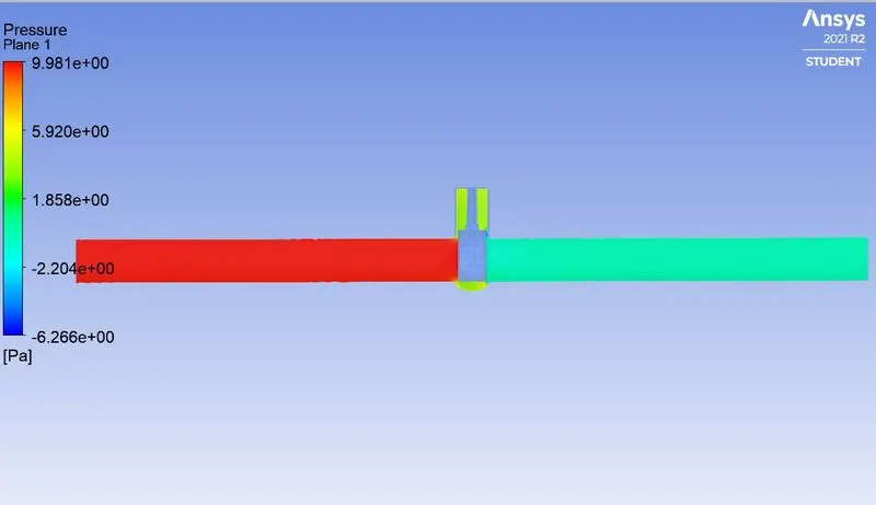
Pressure Contour -

                                   
5.4.1] Parametrization of Valve Lift -
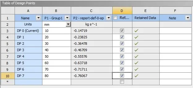
*Close fluent and go back to project schematic ,we can see new option has been added at the bottom of the fluent window,named as 'Parameters'.
*Double click on it.We can see on the right hand side a table consisting of design points and there is a empty row there.
*In the row below 10 mm add values from 20 to 70 and click on update design points.
*To view the updated geometry,meshing,solution data,animations,contours etc of newly created design point,click on retain data.
*After updating design points we can see the values for mass flow rate for each design point.
*To see the individual solution for a perticular design point,right click on it and select set as current.

                         

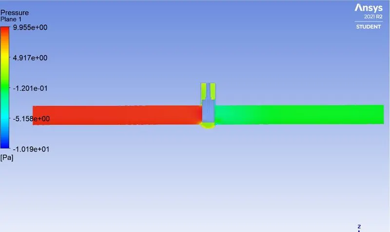
5.4.2] Mass Flow Rate plot and Velocity contour for valve lift = 20 mm -

Mass Flow Rate Plot-
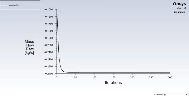
*We can see from the below plot,we are getting a good conserved value for mass flow rate.From the console we can see that
mass flow rate value is `-0.23825``(kg)/s` .The negaive sign indicates that mass flow is leaving the domain.

                                  
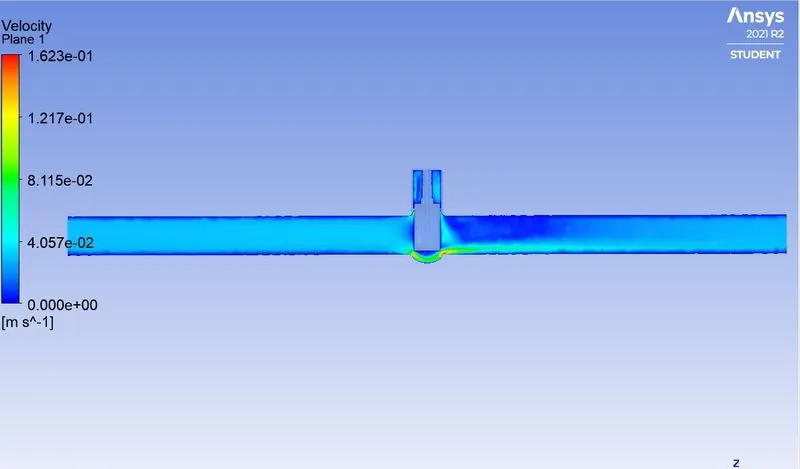
Velocity Contour -

                                   
Pressure Contour -

                                   

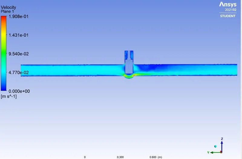
5.4.3] Mass Flow Rate plot and Velocity contour for valve lift = 30 mm -

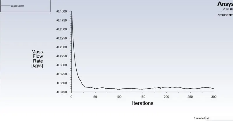
Mass Flow Rate Plot-
*We can see from the below plot,we are getting a good conserved value for mass flow rate.From the console we can see that
mass flow rate value is `-0.36478``(kg)/s`.The negaive sign indicates that mass flow is leaving the domain.

                                 
Velocity Contour -

                                
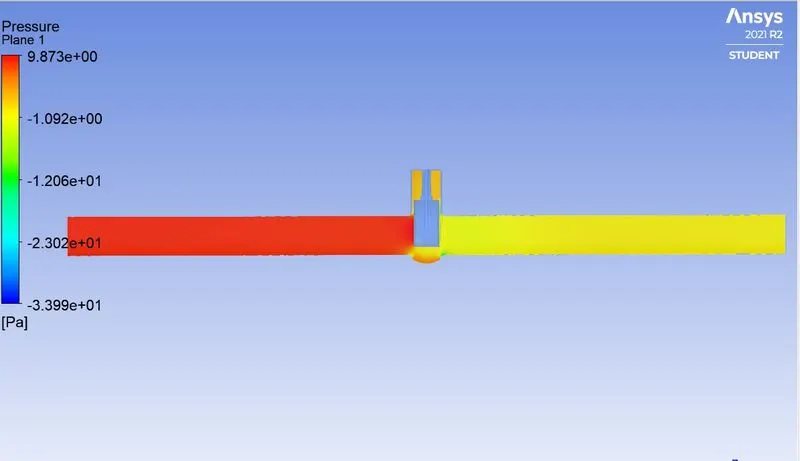
Pressure Contour -

                               

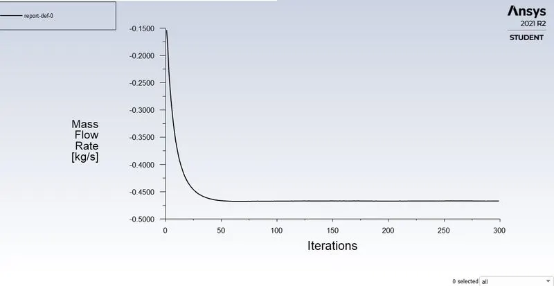
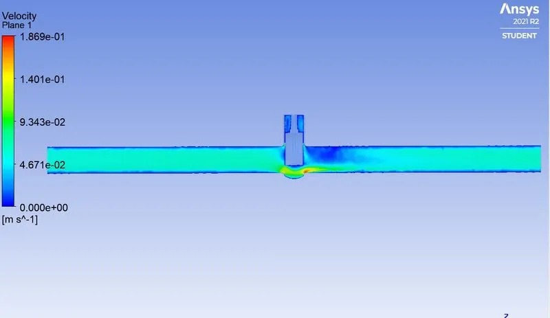
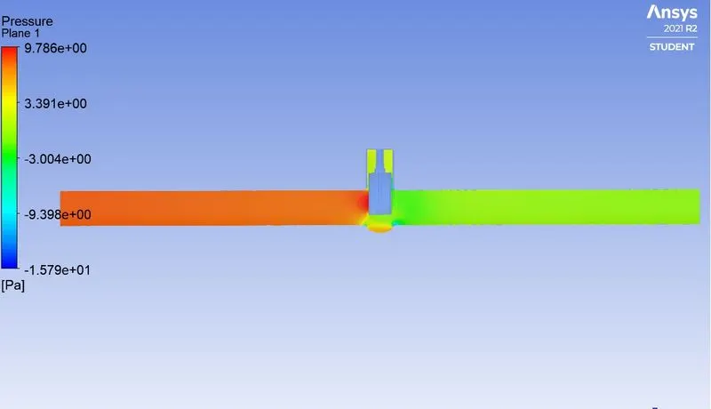
5.4.4] Mass Flow Rate plot and Velocity contour for valve lift = 40 mm -

Mass Flow Rate Plot-
*We can see from the below plot,we are getting a good conserved value for mass flow rate.From the console we can see that
mass flow rate value is  -46709 `(kg)/s` .The negaive sign indicates that mass flow is leaving the domain.

                               
Velocity Contour -

                               
Pressure Contour -

                               

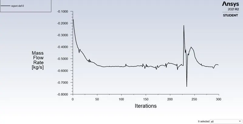
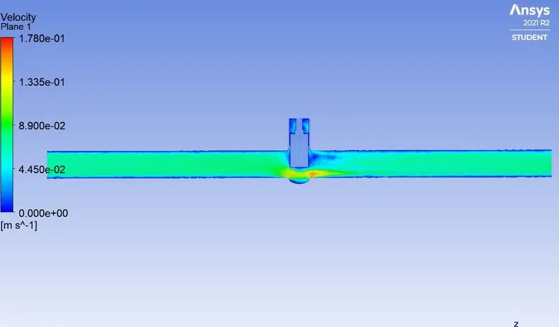
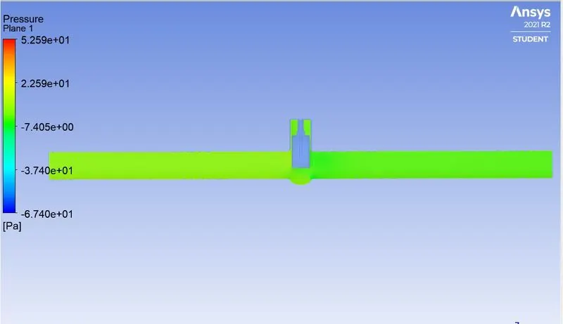
5.4.5] Mass Flow Rate plot and Velocity contour for valve lift = 50mm -

Mass Flow Rate Plot-
*We can see from the below plot,we are getting a good conserved value for mass flow rate.From the console we can see that
mass flow rate value is  -0.55576 `(kg)/s` .The negaive sign indicates that mass flow is leaving the domain.

                              
Velocity Contour -

                               
Pressure Contour -

                               

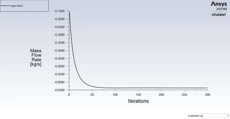
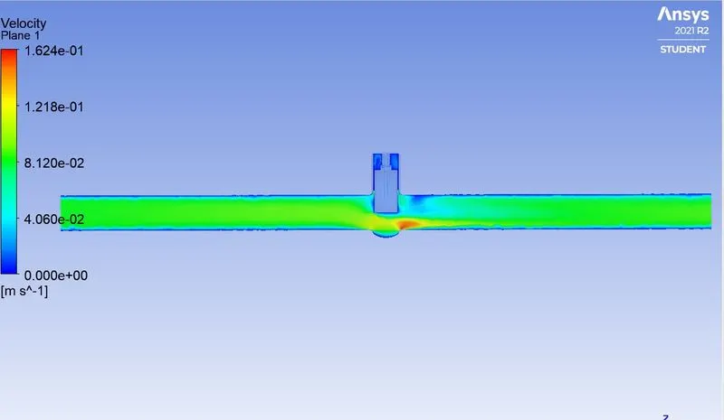
5.4.6] Mass Flow Rate plot and Velocity contour for valve lift = 60 mm -

Mass Flow Rate Plot-
*We can see from the below plot,we are getting a good conserved value for mass flow rate.From the console we can see that
mass flow rate value is  -0.63718 `(kg)/s` .The negaive sign indicates that mass flow is leaving the domain.

                             
Velocity Contour -

                             
Pressure Contour -

                              

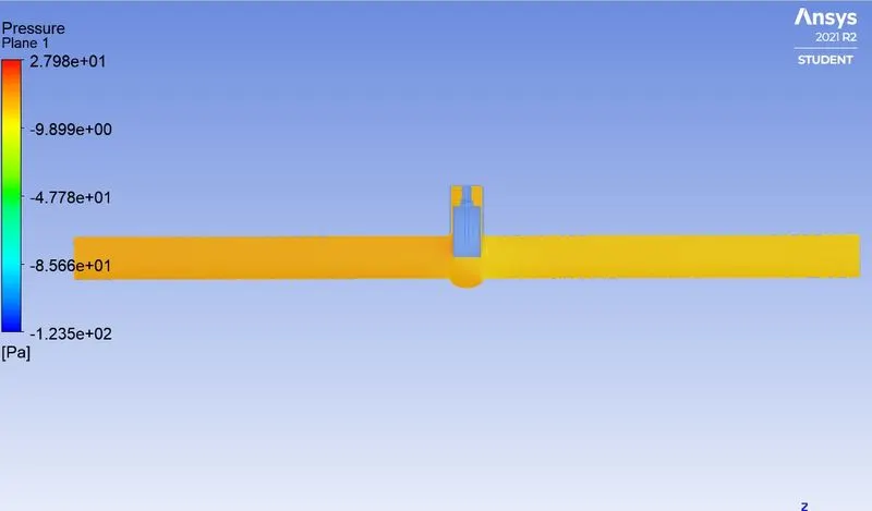
5.4.7] Mass Flow Rate plot and Velocity contour for valve lift = 70 mm -

Mass Flow Rate Plot-
*We can see from the below plot,we are getting a good conserved value for mass flow rate.From the console we can see that
mass flow rate value is  -0.71711 `(kg)/s` .The negaive sign indicates that mass flow is leaving the domain.

                             
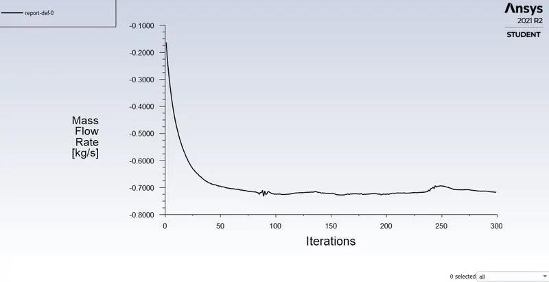
Velocity Contour -

                              
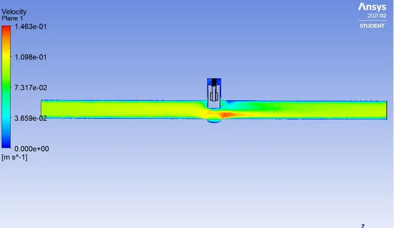
Pressure Contour -

                              

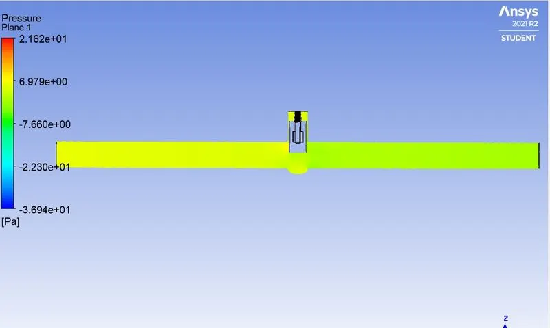
5.4.8] Mass Flow Rate plot and Velocity contour for valve lift = 80 mm -

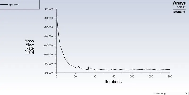
Mass Flow Rate Plot-
*We can see from the below plot,we are getting a good conserved value for mass flow rate.From the console we can see that
mass flow rate value is  -0.76066 `(kg)/s`.The negaive sign indicates that mass flow is leaving the domain.

                             

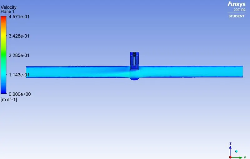
Velocity Contour -

                             

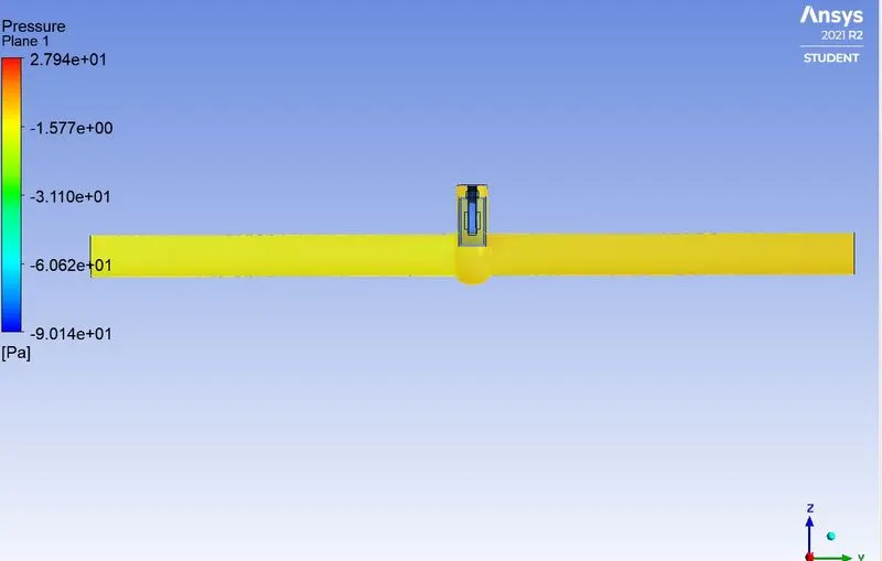
Pressure Contour -

                           

6] Calculation of Flow Coefficient and Flow Factor for different Valve Height -

Q(total) = 1 `(kg)/s` = 3.6 `m^3/(hr`

Flow Factor  (`K_v`) = `Qsqrt(S_g/(Deltap`  where `S_g =1`

Flow Coefficient (`C_v`) = `K_v/0.865`

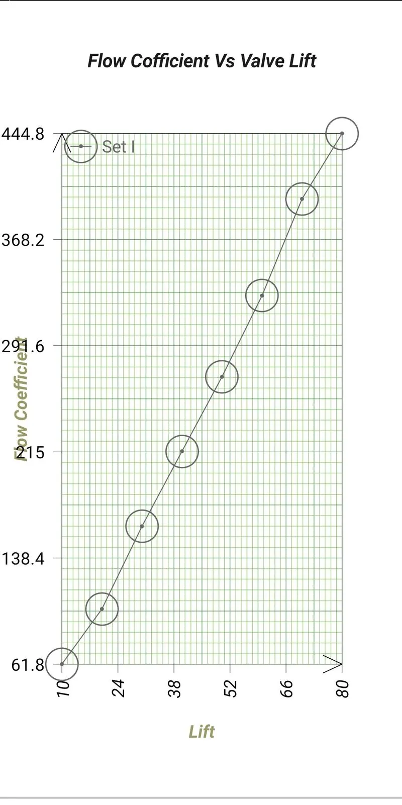
Valve Lift(mm)	Mass Flow Rate(Q)(`m^3/(hr)`	Pressure Drop(`Deltap`)(bar)	Flow Factor(`K_v`)	Flow Coefficient(`C_v`)
10	0.52988	0.000098148	53.48599	61.83351
20	0.8577	0.000095167	87.92091	101.64267
30	1.31320	0.000088585	139.52544	161.30109
40	1.68152	0.000081431	186.34089	215.42300
50	2.00073	0.000073814	232.87368	269.21813
60	2.29385	0.000065457	283.52322	327.77250
70	2.58159	0.000056345	343.92249	397.59826
80	2.73837	0.000050647	384.78245	444.83520

6.1] Plot of Flow Coefficient Vs Lift -

                                                                                     

6.2] Plot of Flow Factor Vs Lift -

                                                                             

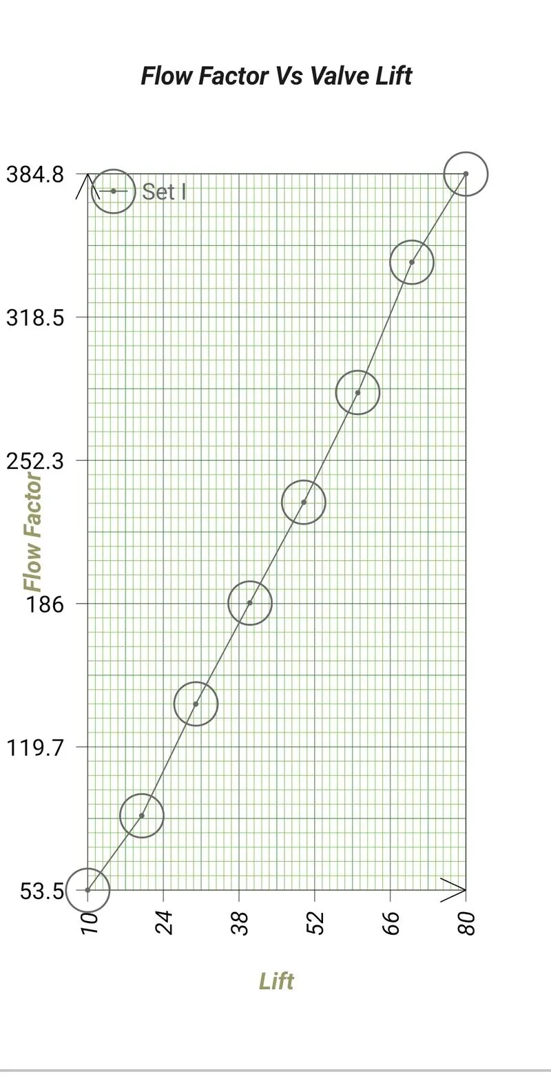
6.3] Compairing results of mass flow rate and flow coefficient for increasing lift -

*We can observe from the result that,with increasing valve lift there is increase in mass flow rate and also decrease in
levels of pressure drop.
*As the flow rate is increased,flow coefficient also increases.And at the same flow rate,higher flow coefficient means lower
pressure drop across the valve.

7] Conclusion -
*As the mass flow increases so does the flow coefficient.And pressure drop decreases.
*So when selecting the valve,for low pressure drop, flow coeffcient should be high enough to suit the specific operating conditions.