Week 4 - CHT Analysis on Exhaust port
1) .Aim -
To perform CHT analysis on an exhaust port.
2). Objective -
1. Give a brief description of why and where a CHT analysis is used.
2. Maintain the y+ value according to the turbulence model and justify the results.
3. Calculate the wall/surface heat transfer coefficient on the internal solid surface and show the velocity and temperature
contours in appropriate areas.
4. How would you verify if the HTC predictions from the simulations are right ? On what factors does the accuracy of the prediction depend on ?.
3). Theory and Introduction -
The term conjugate heat transfer can be used to describe the process which involve a temperature variation within the solids
and fluids itself due to the thermal interaction between the solid and the fluid.During CHT the heat transfer can take place
from solid media to the fluid media and vice versa.This is because fluid flow around solids or between solid walls,and also
the solids are mostly immersed in a fluid.CHT involves heat exchange that occurs simultaneouly by convection between a fluid and a adajacent wall and by conduction through the solid.
CHT analysis is beneficial in enigineering applications because it shows the heat exchanging capabilities between two surfaces
in the engineering device and various optimization can be done to improve the thermal characteristics of the devices.Thus,this can be used to improve the heat transfer rate wherever required.It also helps us to identify the key parameters to enhance the fluid flow and heat transfer within the system.
CHT corresponds with the combination of heat transfer in solid and fluid.In solids conductions dominates while in fluids
convection dominates.Efficiently combining heat transfer in fluids and solids is the key to designing effective coolers,
heaters or heat exchangers.The forced convection is the most common way to achieve high heat transger rate.In some applications performance is further improved by combining convection with phase change.CHT can be performed to improve the cooling performance of water jackets and increase the engine life.
In this study,our objective is to simulate the flow through an exhaust manifold.As the heated fluid flow is going through manifold, it is going to exchange heat with the solid,we want to simulate that process.We will be doing this by assuming that ,initially flow is coming from the exhaust,which is basically through all the four inlets.Also will assum that the flow is really hot and thats going to heat the pipe from inside and on surface we are going to assume that there is a perticular heat transfer.The heat transfer coefficient on the outer surface is depend on the reynolds number of the outside air in contact with the pipe outer surface,we will give it as input here i.e. heat transfer coefficient for the outer wall boundary condition.
4). Solution Procedure -
For solving the CHT analysis on exhaust port,we will follow the below procedure :-
Geometry Creation --> Meshing --> Setup --> Solution & Post Processing
4.1). Geometry Creation -
* Launch the Ansys workbench.First drag and drop the Fluid Flow(Fluent)model into project schematic and double click on geometry to launch the SpaceClaim.
* Import the geometry in to the ansys spaceclaim.
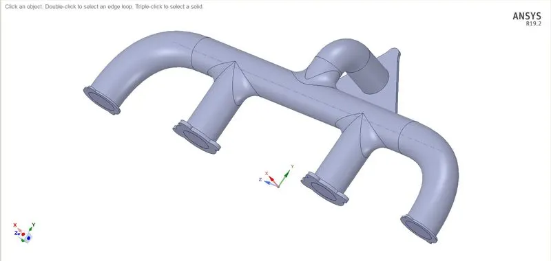
* First we need to check the geometry for any extra edges.To do that,click Repair => extra edges => remove all the red entities => ok .
* Since geometry has solid parts,we need to extract fluid volume,for that follow the below procedure,
click Prepare => volume extract => select edge selection => select all inlet & out let edges => ok.
* Now change the name of the fluid into fluid volume and solid into solid volume.
* Before going into meshing we need to make sure that the mesh which we will generate is a conformal mesh.
* Conformal mesh means the vertex of solid volume should be connected to the vertex of the fluid volume and perticular face of the fluid volume should be connected to the respective face of the solid volume.
* But before this,we need to combine both the components into single one. select both solid & fluid volumes => right click => move to new component => name it as final geometry.
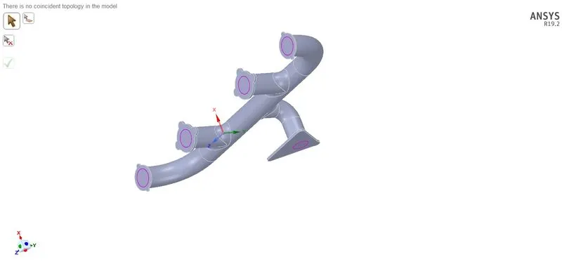
* Now we need to enable share topology in ansys spaceclaim to achieve conformal mesh. click in structure window => FFF => proerties => share topology => share. click workbench => share prep.
4.2). Meshing -
*Now,go to meshing, by double clicking on mesh,and first do the name selection i.e give proper boundary names.Then generate the basic mesh using generate mesh command.We can see the flow of the mesh inside the extracted volume by using section plane.Also we can check the mesh quality by using mesh quality option.
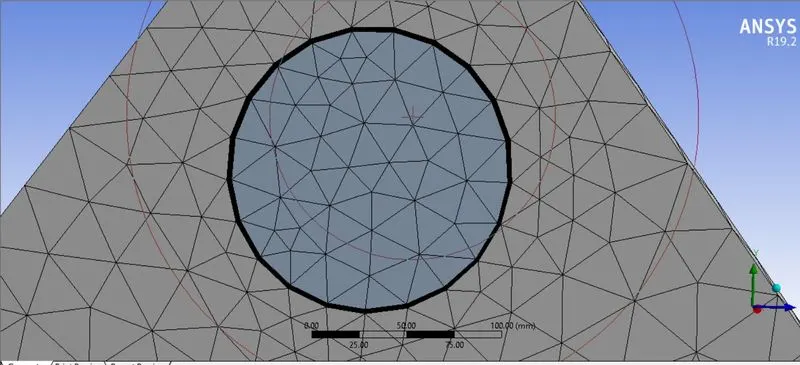
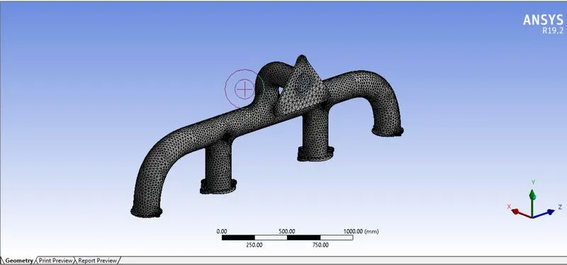
Number of Elements Generated - 375820
*In meshing we can see the mesh is perfect.This is exactly how we need to make meshes for CHT cases.Always create the named selection first ,before generating the mesh.Select the edge you want to name,click N & name the selection.
In similar fassion name our inlets,outlet,and for the outer face double click on the pipe surface,this will select all the necessary pipe surfaces name them as outerwall convection.
*We also have another remaining faces or walls i.e. flange part.
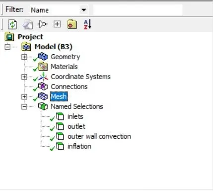
*Ansys mesher automatically import those faces as wall and by deault,these walls will have adiabatic boundary condition i.e.these bodies won't allow any heat transfer to take place.Thats exactly what we want.
*Then,next thing to do is to mesh.We click the mesh option in the side window and create our base line mesh.We then refine mesh.
4.2.1). Inflation -
*Inflation layer helps us to create a body fitted mesh.It means,it creates a layer of mesh same as the geometry.
*Since solid fluid interface is important,it's where we want to calculate heat transfer,so we need to capture it accurately.
*To do this,hide the solid body part,select fluid volume part and name it as inflation layer.
*In global mesh => select inflation => use automatic inflation => all faces in chosen named selection => named selection => inflation layer.
*For inflation option,we will use first layer thickness and will give this value based on y+ value.
*Since we are dealing with walls,we will use k-omega SST model.With y+ between 0.1 to 5.
4.2.2). First Layer Thickness -
1) `U_infty` = freestream velocity = 5 m/s
2)`rho` = freestream density = 1.225`( kg)/m^3`
3) `mu` = dynamic viscosity = 0.000017894 `(kg)/(ms`
4) L = Diameter of the inlet (m) = 0.1662206 m
5) desired y+ = 1
Reynolds number = Re = `(rho*U_infty*L)/mu`
= `(1.225*5*0.1662206)/0.000017894`
=56896.2319
Skin friction coefficient = C_f = `0.026/R_e^(1/7)`
=`0.026/(56896.2319)^(1/7`
= 0.00544096214
Wall shear stress = `tau_(wall) = (C_f*rho*U_infty^2)/2`
=`(0.00544096214*1.225*(5)^2)/2`
= 0.08331473276
Friction velocity = `U_f = (tau_(wall)/rho)^(1/2)`
= `(0.08331473276/1.225)^(1/2`
= 0.26079115541
Hence,
First layer thickness, `Deltas = (y+*mu)/(U_f*rho)`
= `(1*0.000017894/( 0.26079115541*1.225))`
= 0.0000560116653 m
= 0.0560116653 mm
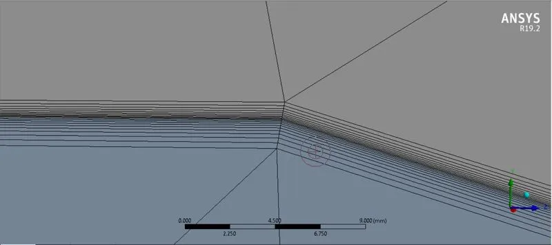
* Insert the calculated first layer thickness,and maximum of 10 growth layers with growth ratio of 1.2.
* Generate mesh & will get inflation layers generated.
4.3). Sizing(Body sizing) -
*Now we will make mesh finer for fluid volume.
Right click mesh => sizing => in geometry select inner fluid volume by hiding outer body & give size 20 mm => generate mesh.
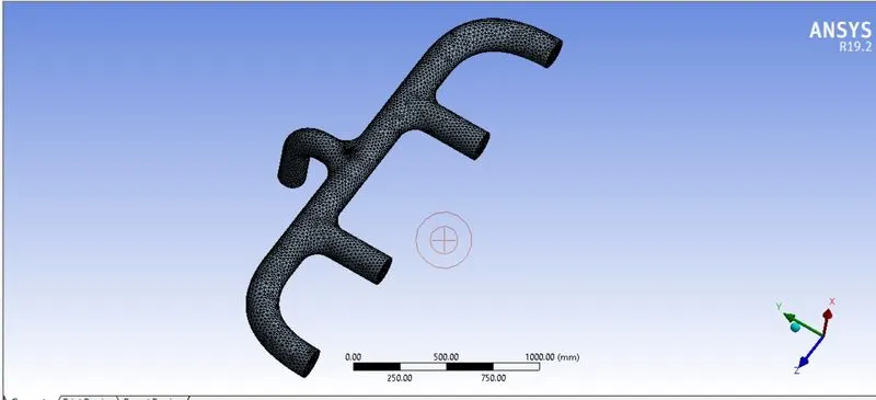
*Simillarly mesh outer body and make sure to turn on capture curvature.
* Now lets check our mesh quality.Our minimum mesh quality is good enough.
* This concludes our meshing procedure.
* Now close the mesh & update.
4.4). Setup -
* Double click setup in project schematic.This will open ansys fluent.
*Click on check mesh and make sure there are no errors.
4.4.1). Setting up Physics-
Our solution method will be SIMPLE.
We need to enable energy to capture temperature.
4.4.1.1). General -
*Solver type - pressure based
*time - Steady state
*velocity formulation - absolute

4.4.1.2). Models -
*viscous model - k-omega SST
4.4.1.3). Material -
*Fluid - Air
*Solid - Aluminium
4.4.1.4). Zones -
Cell zone - In cell zone we can see our fluid volume ,Set it to fluid type,with material air and solid volume set it to solid type
material aluminium.
4.4.1.5). Boundary conditions - We can see all the named selections which,we generated above being used as boundary conditions.
* A) Inlet -
Type - velocity inlet
velocity magnitude - 5 m/sec
Temperature - 700k
* B) Outlet -
Type - pressure outlet
gauge pressure - 0 Pa
* C) Outerwall convection -
Type - wall
Thermal conditions - convection
Heat transfer Coefficient - 20 `W/(m^2K`
* D) Flanges and support -
Type -wall
Thermal conditions - Heat Flux
Heat Flux - 0 `W/(m^2K`(Adiabatic walls)
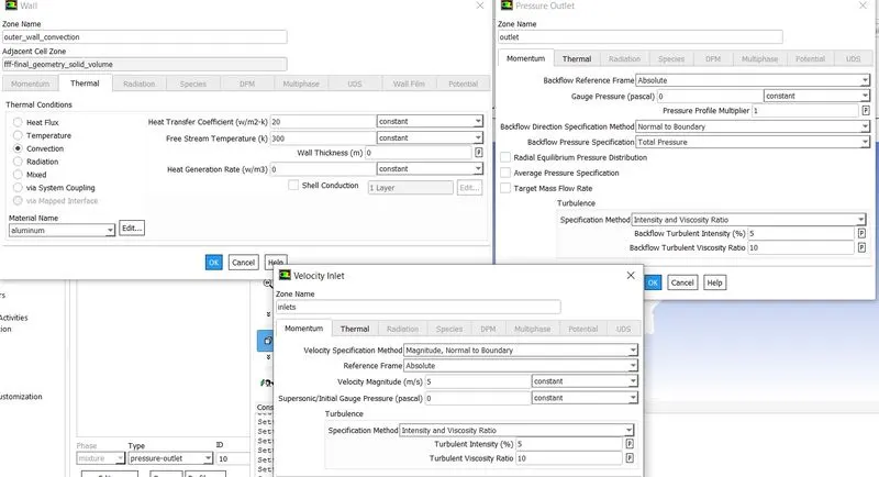
*Now initialize the domain.We will use hybrid initialization,this provides very good initial conditions.
*We want to moniter different flow quantities as the solution is being generated,will use contours for this.We want to see how
the velocity and pressure & temperature variation looks like.
For temperature go to postProcessing => contours => new => contour of => Temperature => under it static temperature => select outerwall & hit save/display.Simillarly create contour for velocity and pressure.
*To create animation,go to activities => solution animation => select temperature contour => preview => set desired view => give name as temperature animation.
4.5). Solving -
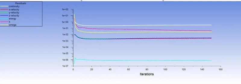
* We will run the simulation for 200 iterations.We can see from the residual plot that our solution has converged and reached the steady state.
5). Results -
5.1). Residual Plot -
*It can be observed from the residual plot that solution remain unchanged after 120 iterations.
5.2). Temperature Contour -
*Below is the plot for temperature contour.
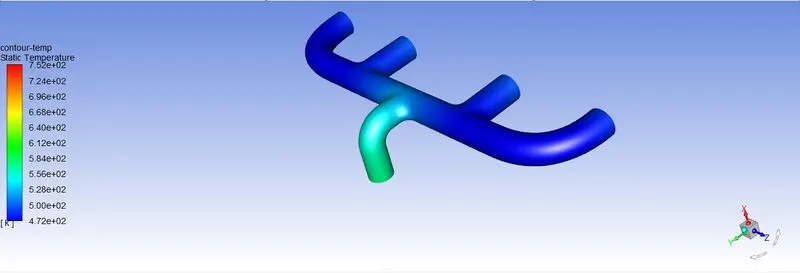
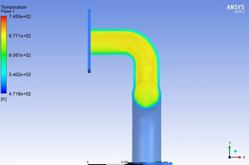
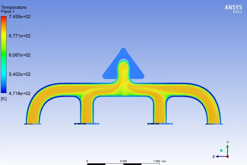
*Now if we look at the results,we can see that,there is less temperature right after inlet ports and are getting more temperature at outlet port.The reason for this is convection.To explain this lets look at the stream lines.
5.3). Streamlines Plot -
*To plot streamlines ,click streamlines => keep default name => in geometry => start from inlet.
*Below is the streamlines plot,colored with velocity .
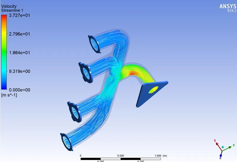
*Here we have 4 inlets and 1 outlet.We know that mass flow rate must be conserved.So since there is only one outlet,velocity at outlet is going to be higher,which means Reynolds number is going to be higher,which also means theres going to be higher heat transfer coefficient,which means theres going to be more heat transfer from fluid to the solid,thats why solid temperature at outlet is high.
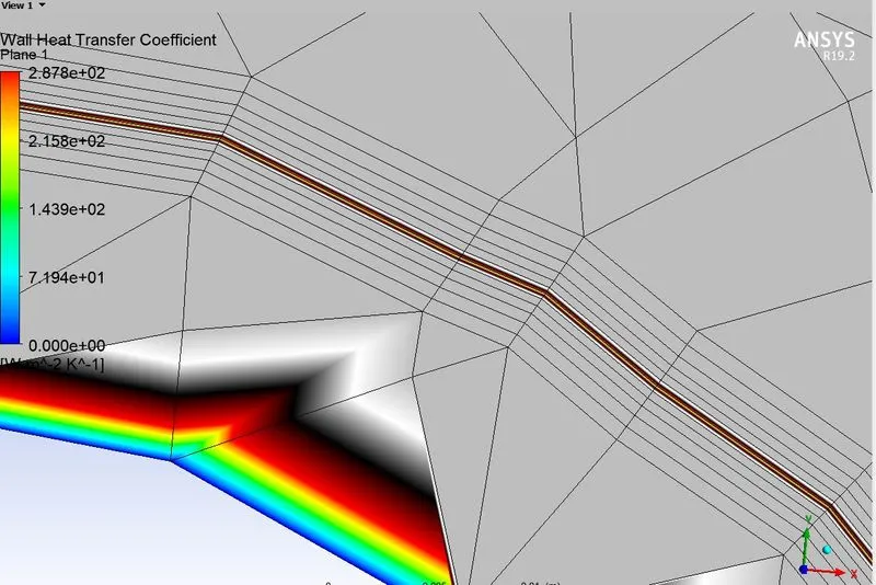
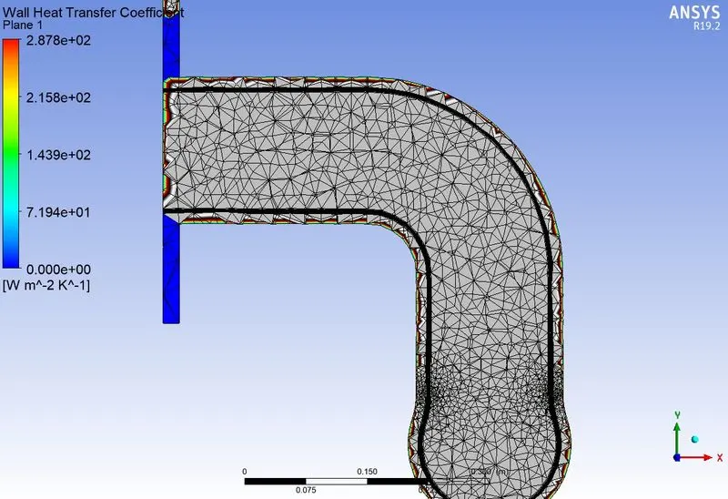
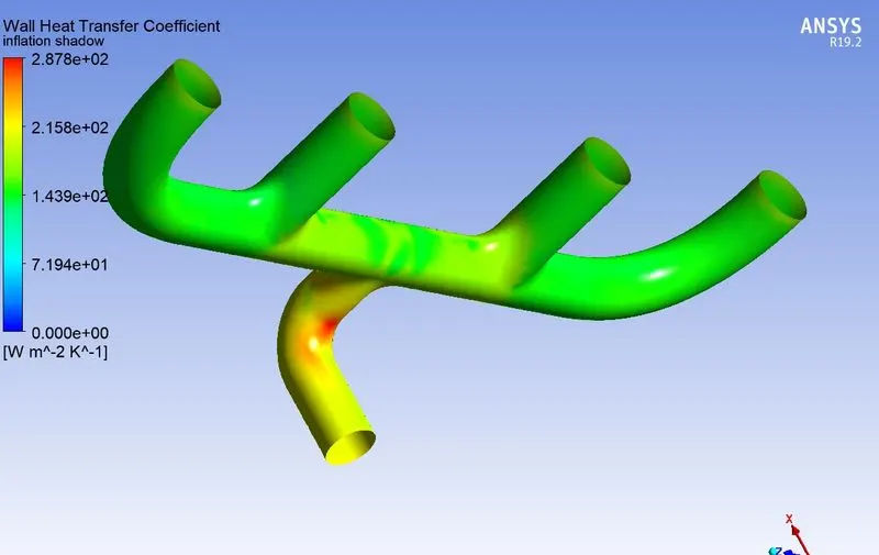
*Let's insert a plane at outlet to show wall heat transfer coefficient,it is the quantity that is only calculated at first cell
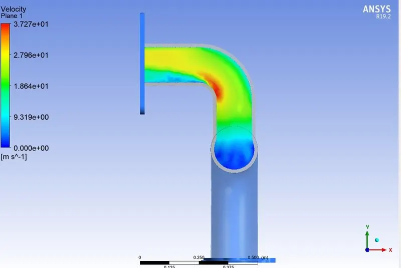
of the wall adjacent to the fluid.If we observe the plot,we can see that heat transfer is high at the curve section in the outlet
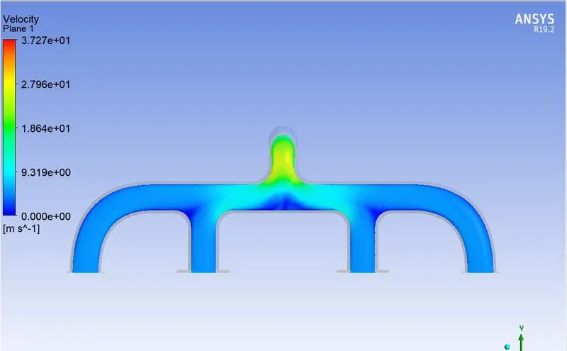
pipe.And also from the velocity contour we can see that,at the same location fluid velocity is high causing high heat transfer.
5.4). Velocity Contour -
*Below is the plot for velocity contour.We can see velocity is higher at outlet pipe.
5.5). Heat Transfer Coefficient Contour -
*Below is the plot for heat transfer coefficient contour.We can see heat transfer coefficient is high at outlet compared to 4 inlets.
 .
. 
5.5.1). Area weighted average value of Surface Heat Transfer Coefficient -
The below image shows area weighted average value of surface heat transfer coefficient on the internal solid surface.The negative sign indicates that heat flux is leaving the surface.

6). Verifying the HTC predictions from the simulations -
*The nusselt number is the ratio of convective to conductive heat transfer across a boundary.
Nu_L = convective heat transfer/conductive heat transfer = hL/k
where, h - convective heat transfer coefficient of the flow
L - Characteriatics length
k - Thermal conductivity of the fluid
Also Nusselt number is releated to Reynolds Number(Re)
`Nu = 0.023Re^(4/5)Pr_n^0.4`
where, Re = uL/nu = rho*uL/mu
u = flow speed (m/s)
* If we observe heat transfer coefficient is directly proportional to the reynolds number(also to the velocity).So if you increase the velocity then there will be increase in the convective heat transfer coefficient.Thats what we have proved above.Also if we run another simulaton and increase reynolds number ,the heat transfer coefficient will increase.
6.1)Compairing Numerical With Analytical HTC value -
HTC = h = `(N_u*k)/L`
Since ,
`Nu = 0.023Re^(4/5)Pr_n^0.4`
`P_r=C_p*mu/k`
`C_p=1006`
k = `0.0242 w/(mk)`
Therefore,
`P_r = (1006*1.7894*10^-5)/0.0242`
= 0.744
`N_u = 0.023*56896.23^0.8*0.744^0.4`
`N_u=130.141`
Therefore,
`h=(130.141*0.0242)/0.16611`
h = 18.96
| Numerical Value | Analytical Value | Error | |
| Heat Transfer Coefficient | 21.22 | 18.96 | 10.650 |
7). Factors on which the accuracy of the prediction depends on -
*Need to choose the exact turbulence model.Since this study is wall boundes,it's best to use k-omegaSST model.
*Share topology should be set to share,to have conformal meshing for proper connectivity.
*Need to give exact heat transfer coefficient for the outer boundary.
*Whenever inputing any values,give proper decimal values to avoide round off error.
*Set proper y+ value based on the turbulence model selected.
8). Conclusion -
*We have successfully performed, the CHT analysis on exhaust port.
*Verified our results using Nusselt number and Reynolds number relation.
*The heat transfer is more at the bend and in the outlet section,because as density and cross section area is constant,flow velocity is increasing to maintain the conservation of mass flow rate,which in turn increases the Reynolds number hence increasing Nusselt number and heat transfer.