Week 6: Conjugate Heat Transfer Simulation

AIM :

To perform conjugate heat transfer simulation on a pipe flow using Converge CFD.

OBJECTIVE ;

*Setup a CHT simulation for a flow through pipe at Reynolds Number(Re)=7000
*Plot the temperature and velocity contour
*Perform grid dependence test.

INTRODUCTION AND THEORY :

The conjugate heat transfer analysis type allows for the simulation of heat transfer bwtween solid and fluid domains by exchanging thermal energy at the interfaces between them.Typical applications of this analysis type exist as,but are not limmited to,the simulation of heat exchangers,cooling of electronic equipments,and general-purpose cooling and heating systems.

CHT analysis is beneficial in enigineering applications because it shows the heat exchanging capabilities between two surfaces
in the engineering device and various optimization can be done to improve the thermal characteristics of the devices.Thus,this can be used to improve the heat transfer rate wherever required.It also helps us to identify the key parameters to enhance the fluid flow and heat transfer within the system.

CHT corresponds with the combination of heat transfer in solid and fluid.In solids conductions dominates while in fluids
convection dominates.Efficiently combining heat transfer in fluids and solids is the key to designing effective coolers,
heaters or heat exchangers.The forced convection is the most common way to achieve high heat transger rate.In some applications performance is further improved by combining convection with phase change.CHT can be performed to improve the cooling performance of water jackets and increase the engine life.

MODELLING APPROACH :

We will consider a fluid flow through a pipe of some thickness.Then will provide some heat flux to the outer pipe surface and will moniter how heat gets transferred in the fluid.

SOLUTION PROCEDURE :

To perform CHT on a pipe flow ,we will follow the below procedure :-

Geometry Creation --> Case Setup --> Solution --> Post Processing

Geometry Creation :

* Launch Converge and start a new project.
*Create the geometry by following below steps,
Create => cylinder => give radius and length and apply => now create another cylinder with slightly more thickness(radius) and same length and apply.
*Now we need to clean the geometry,
Repair => Delete => select triangles and delete intersecting triangles from front and back face.
*Now we need to create triangles,reate triangles using open edge tool and also patch front and back face.
* In converge ,geometries are represented as triangles.So we need to group these triangles to create boundaries.This is the
fundamental step in Converge.
Geometery => Boundary => Flag => click on add and add 5 boundaries => rename first boundary as solid outer wall => using by angle triangle selection,select outerwall triangles => apply.
* Simillarly flag outlet,solid_side,inlet,and interface.

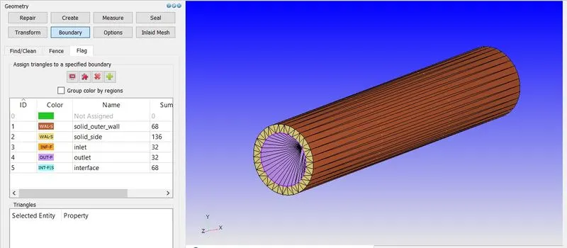
* As our flow is internal,we want all the normals to point into the fluid domain.To do that,
click on normal toggle => transform => normal => click on triangle with outside pointing normal => apply

* Make sure that geometry is clean,
Diagnosis => find => no errors.

CASE SETUP :

* Click on Begin Case Setup => General Flow => Done.

* Our working fluid will be air .
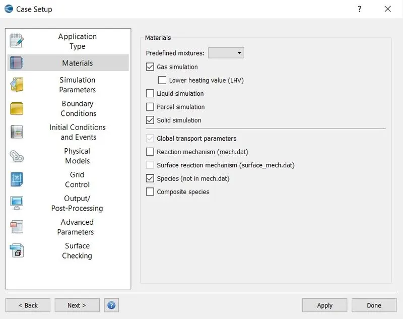
* Materials => Predefined mixture => Air => uncheck reaction mechanism => check gas and solid simulation => check species => Apply & Done.

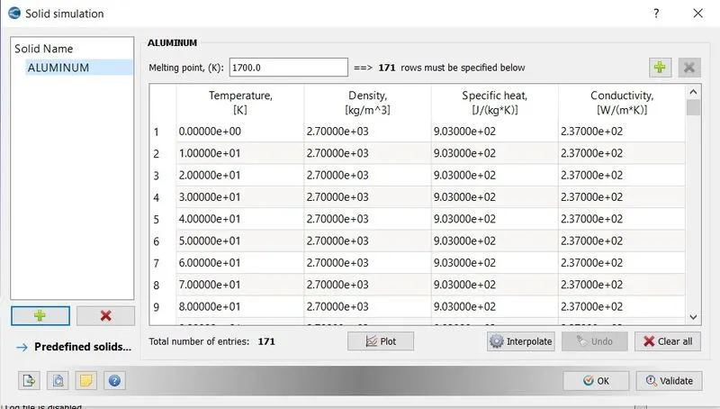
*In solid simulation add aluminium as material.

* Keep default global transport parameters.

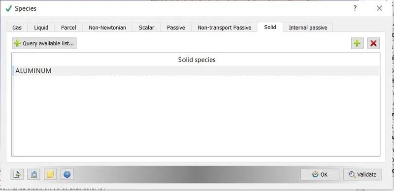
* In species for gas add oxygen and nitrogen and for solid select aluminium.

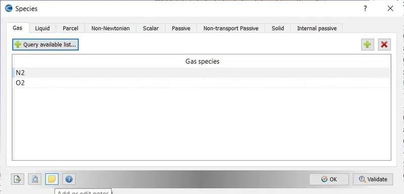
* We will be running transient simulation.To set this follow below steps,
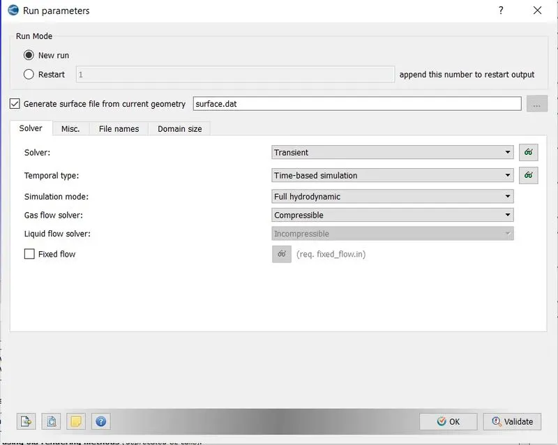
a] Run Parameters => Solver => select transient solver => simulation mode full hydrodynamic => Gas flow solver compressible.

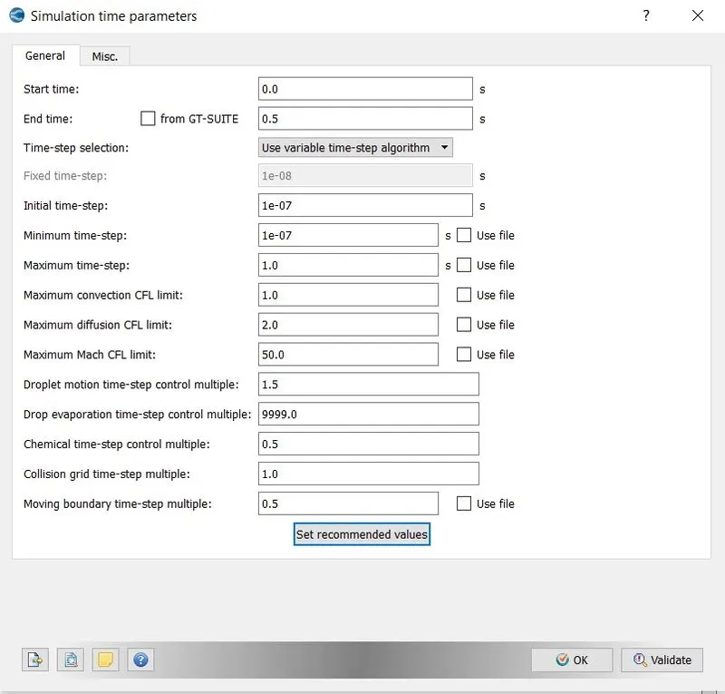
* SIMULATION TIME PARAMETERS =>

Start Time - 0 sec
End Time - 0.5 sec
Initial Time Step - 1e-7 sec.
Minimum Time Step - 1e-7 sec.
Maximum time step - 1 sec.
Maximum Convection CFL limit - 1.0.

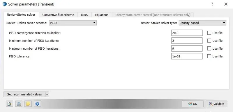
* SOLVER PARAMETERS =>

Navier-Stokes solver Scheme => PISO
Navier-Stokes solver Type => Density Based

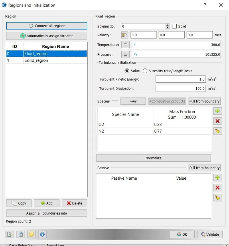
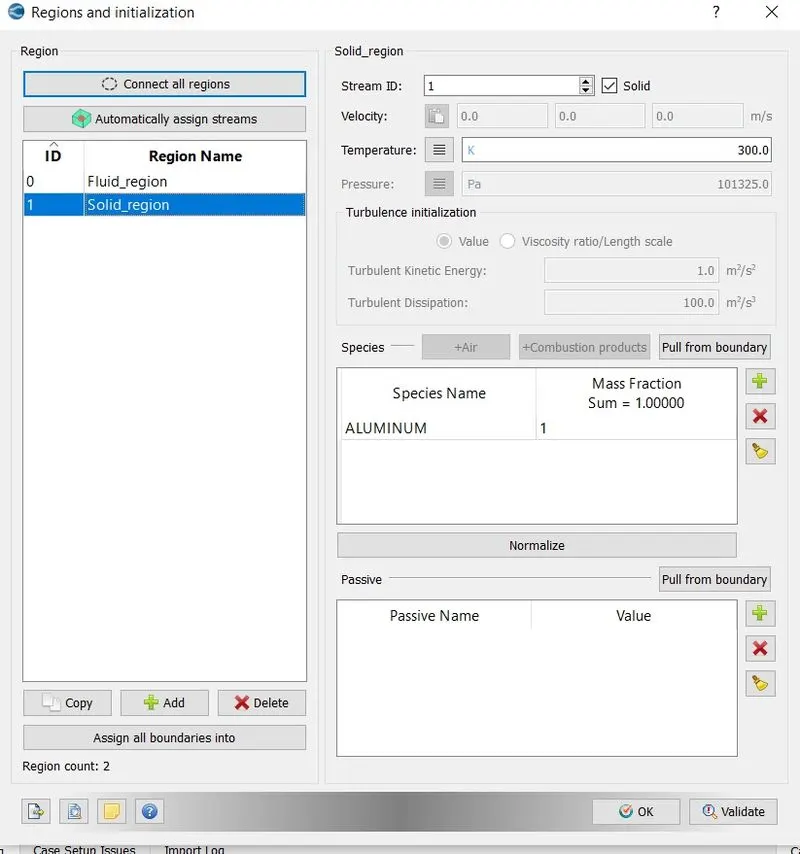
* Now before setting the boundaries,set solid and fluid region ,initial region and set initial pressure and define air species.This region will be assigned to each boundary.In solid region make sure to set stream id 1 and select solid and aluminium as species.

* BOUNDARIES =>

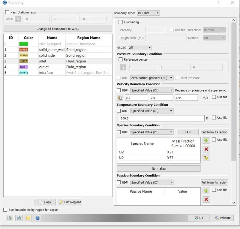
INLET -
Boundary Type - INFLOW
Pressure Boundary Condition - Zero normal gradient(NE)
Velocity Boundary Condition - Specied value = In Z-direction 5 m/s
Temperature Boundary Condition - Specied value - 300 K
Species Boundary Condition - select Air

OUTLET -

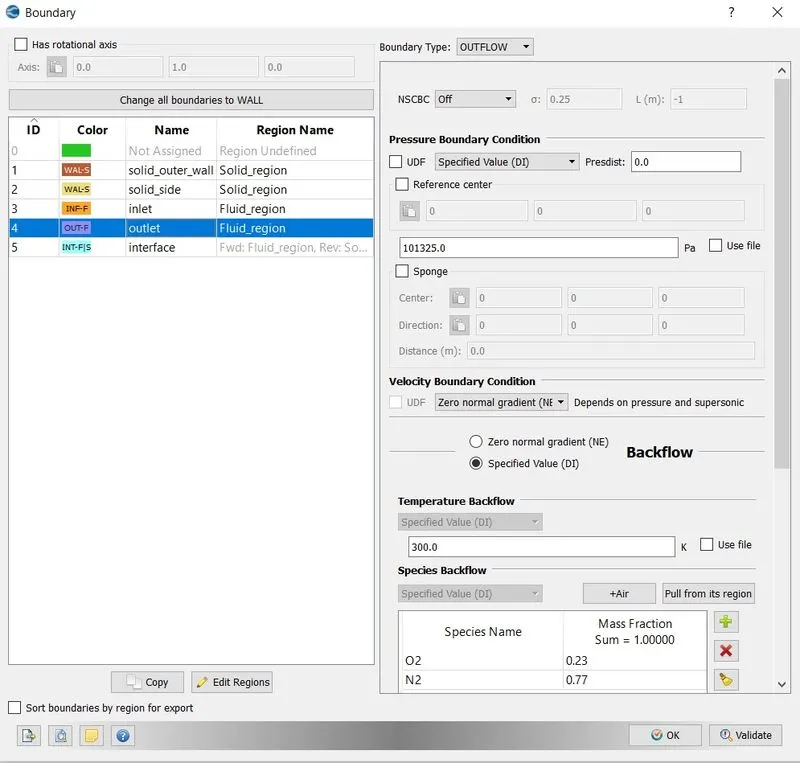
Boundary Type - OUTFLOW
Pressure Boundary Condition - Specied value - 101325 Pa
Velocity Boundary Condition - Zero normal gradient(NE)
Temperature Boundary Condition - Specied value - 300 K
Species Boundary Condition - select Air

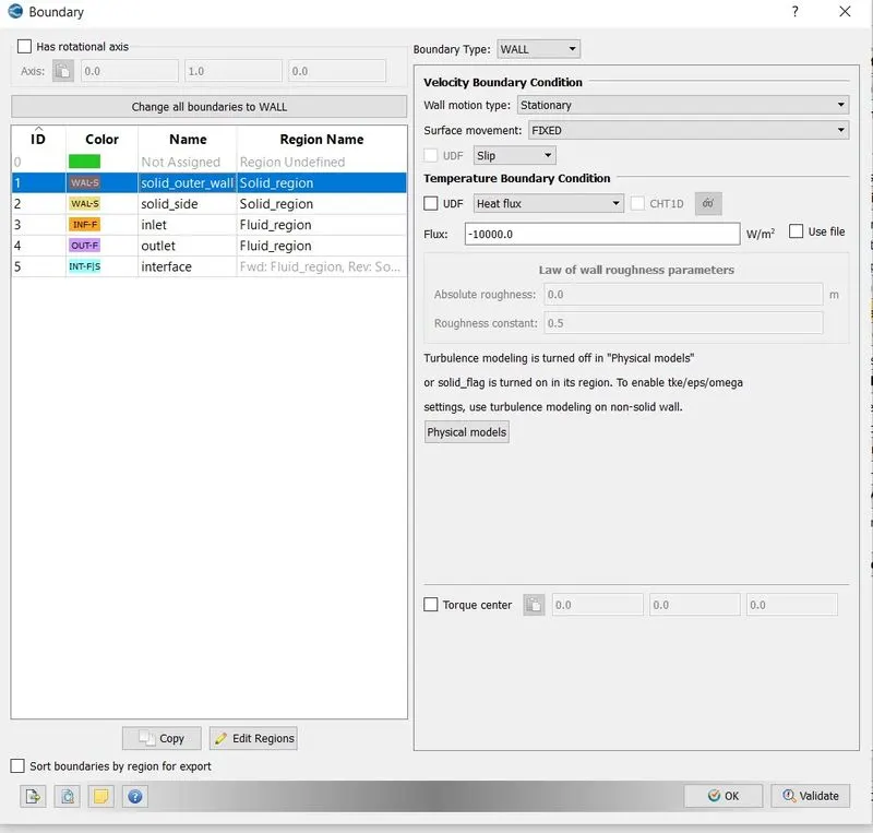
solid_outer_wall(slip) -
Boundary Type - Wall
Wall Motion - Stationary
Surface Movement - Fixed
Temperature Boundary Condition - Heat Flux
Flux = -10000 W/m^2(Negative sign indicates flux entering fluid)

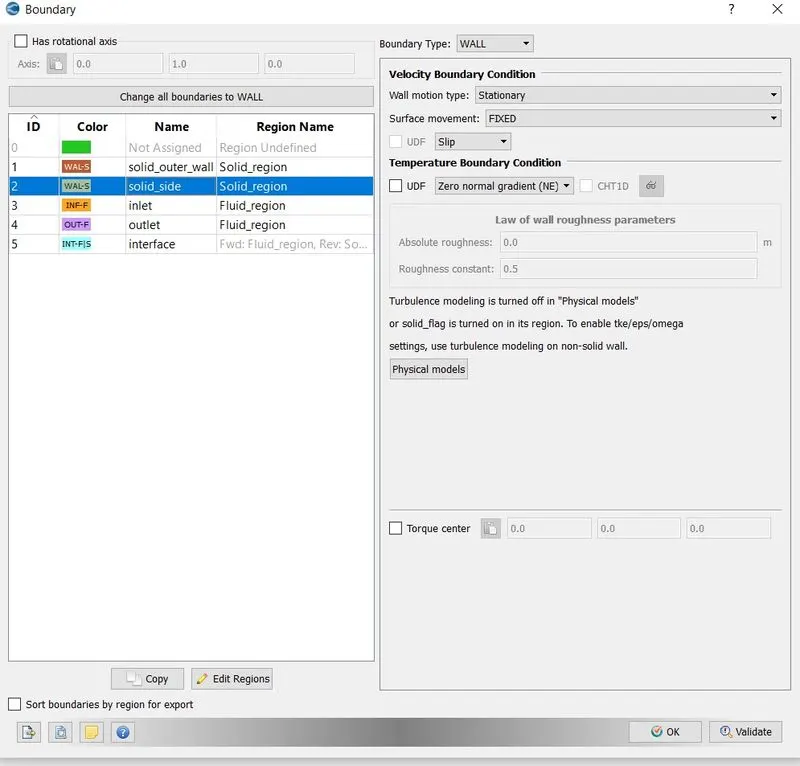
solid_side -
Boundary Type - Wall
Wall Motion - Stationary
Surface Movement - Fixed
Temperature Boundary Condition - Zero normal gradient(NE)

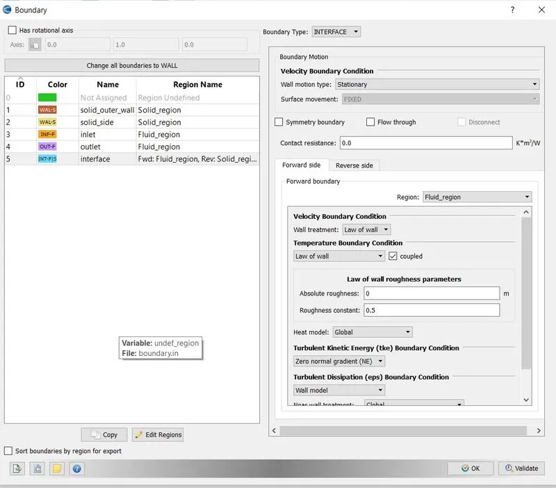
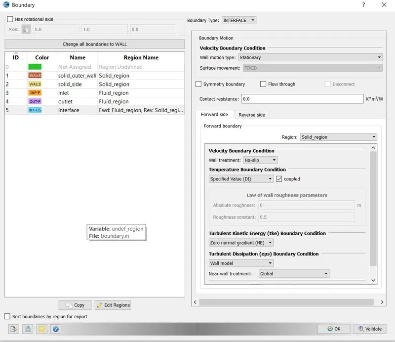
interface -
Boundary Type = INTERFACE

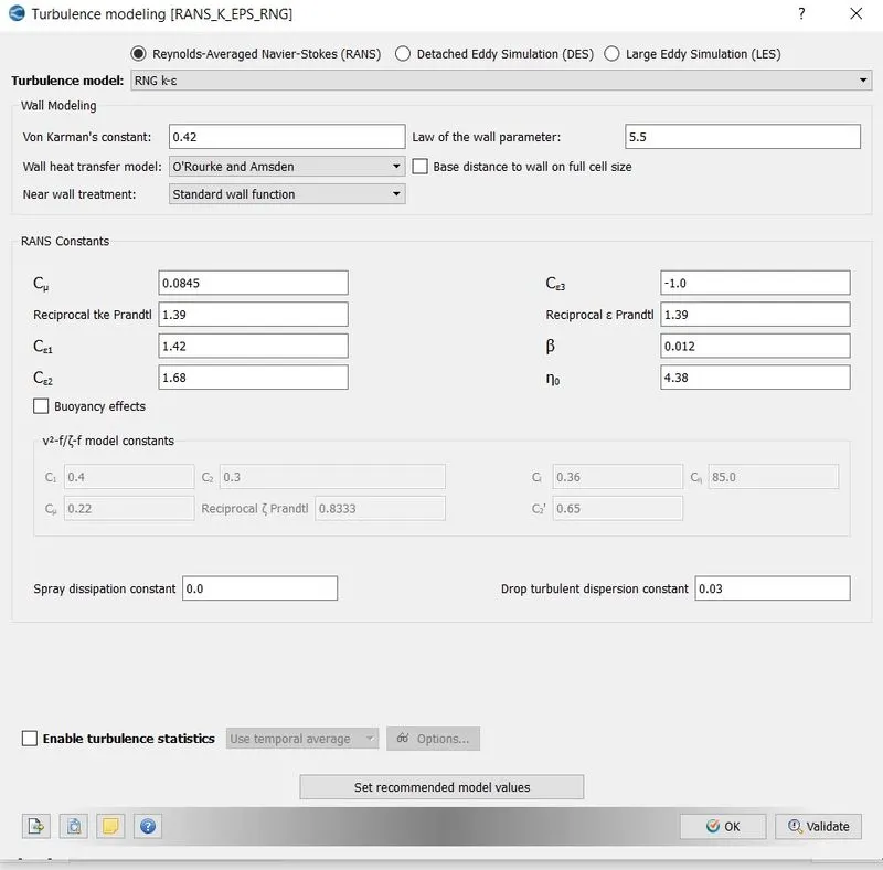
* For turbulence model select RNG k-epsilon.

*SUPER CYCLING
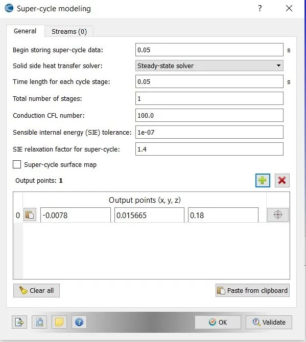
In this fluid and solid are solved together.For solid it is solving the energy equation i.e 3D transient heat conduction equations and for solids it solves Navier Stokes equation.It stores the instantaneous HTcs and temperature on the interface during the simulation process.After some characteristics time it freezes the fluid solver,then time averages heat transfer coefficient and temperature and apply them as boundary conditions at the interface.Solves the solid temperature until it reaches the steady state condition.After that updating the solid temp.field and unfreezes the fluid solver and repeats the procedure until solid temperature converges.

Begin storing super cycle data - 0.05
Solid side heat transfer solver - Steady state solver
Time length for each cycle stage = 0.05
Convection CFL number - 100
Output points = Select output points where you want to moniter variables.

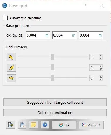
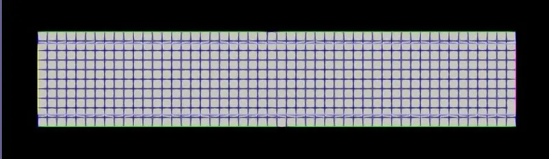
*In converge mesh generation is a fully automatic process.Converge uses cut cell method to generate the mesh.
Base Grid = dx= 0.002 ; dy = 0.002 ; dz = 0.002 => ok

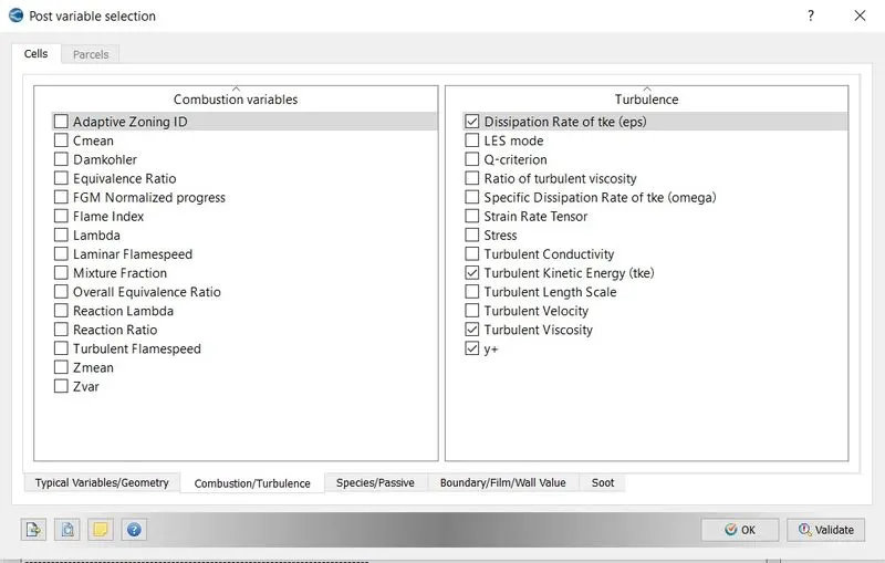
*In post variable selection,select the variables which needs to be post processed and set species mass fraction.

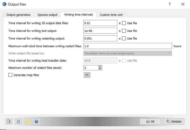
*We want our post processed graphes and animations to be smooth,so we want ample amount of ouput files.It is good practice to have at least 100 3D output files and same amount of text output files.

SOLUTION :

*For running the simulation,first we need to export all the input files to the folder where we want to save our 3D output files,

File => Export => Export Input Files => select the desired folder => Export.

*Now we will use CYGWIN command prompt to run our simulation.But before running the simulation first we need executables which will solve the simulation,for that paste mpiexec.exe and converge.exe into the folder where we have exported all our input files.

*Now using CYGWIN command prompt,navigate to the folder where all the input files are exported,and type the below command,

mpiexec.exe -n 4 converge.exe restricted </dev/null> logfile &

*In the above command ,mpiexec.exe will help us to run our simulation in parallel,-n 4 are the number of cores on which we
want to run our simulation.As we are using the version of converge which has limit on the size of the file it can solve hence the command restricted.And the last part of the command dump all the data that is being generated into the logfile, which we can access during simulation procedure to see where our simulation has reached.

*The above command will create a folder named output containing all the generated 3D output data.As we will be using paraview as the postprocessing tool.Hence we need to convert these output files into the format that paraview can read.For this we will use converge post convert tool.

Go to converge post processing 3D =>give case name => select the file type => navigate to the output folder and select it
=> select all files => select all variables => convert.

This will create group file ,which will be used by paraview to post process our results.

POST-PROCESSING :

Mesh -

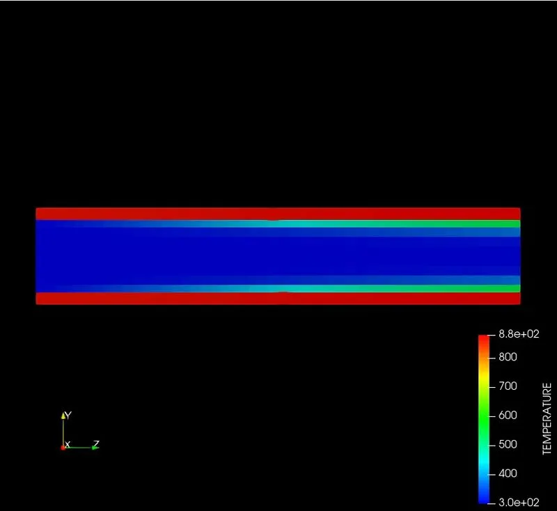
Temperature Contour -

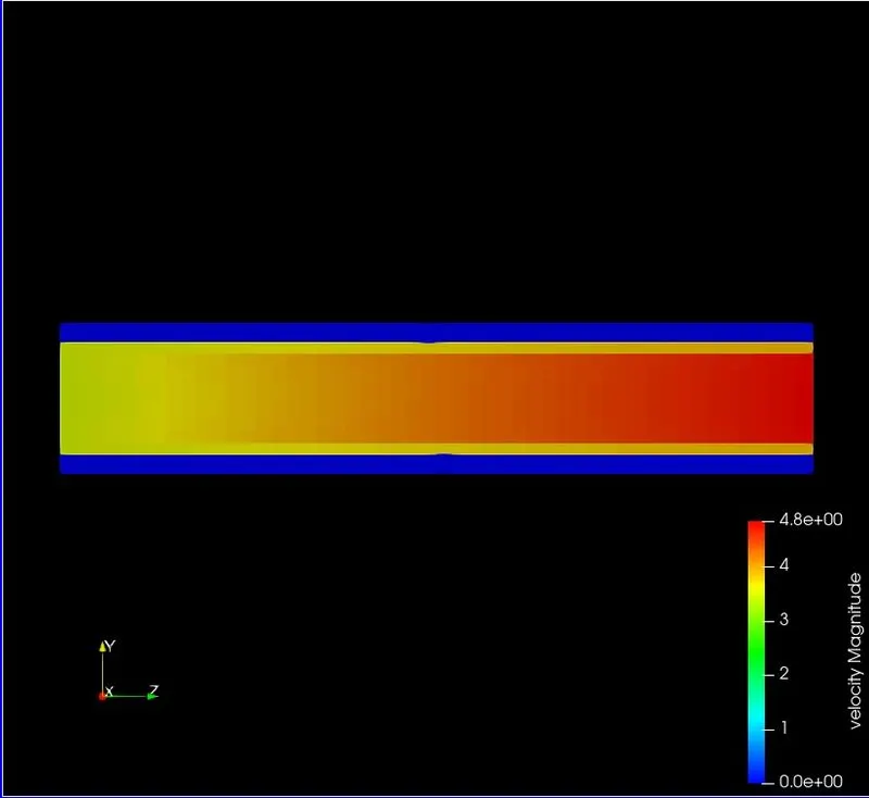
Velocity Contour -

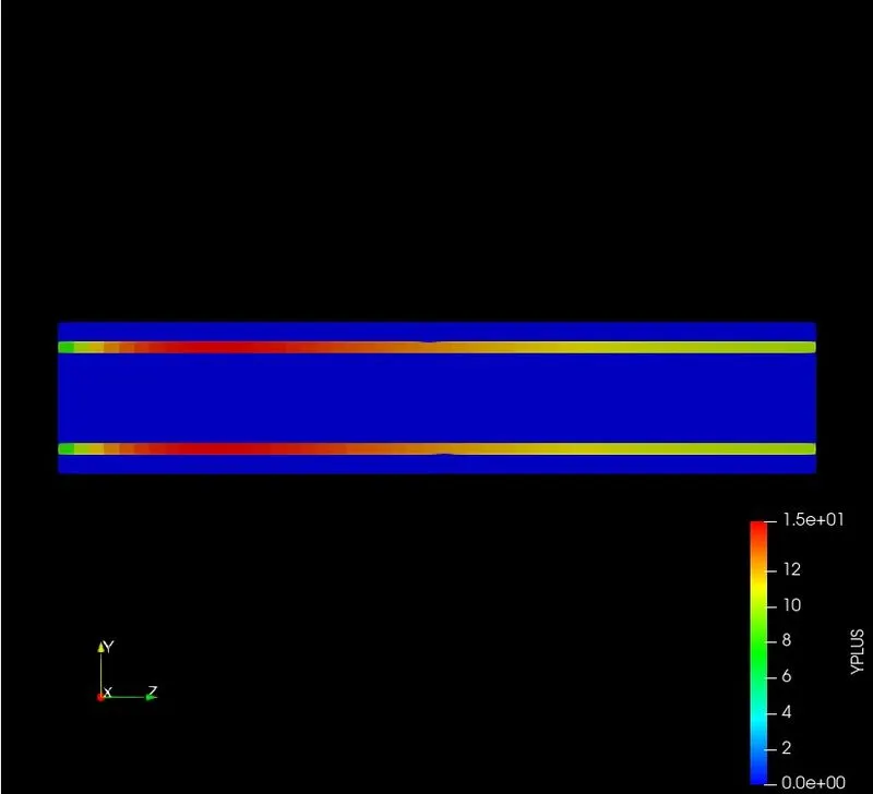
Y+ -

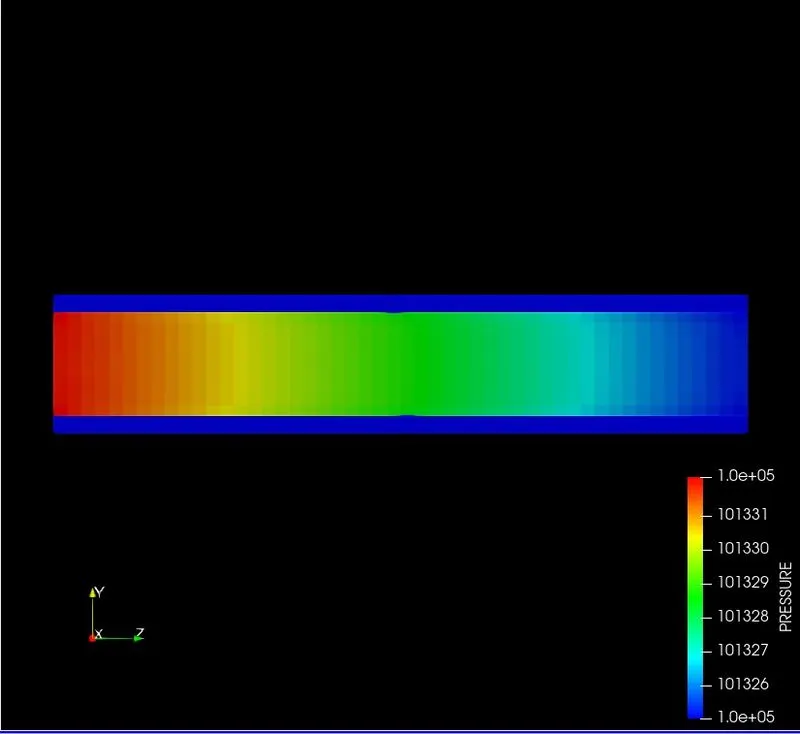
Pressure -

Grid Dependence Test -

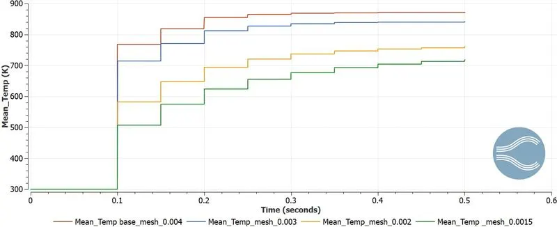
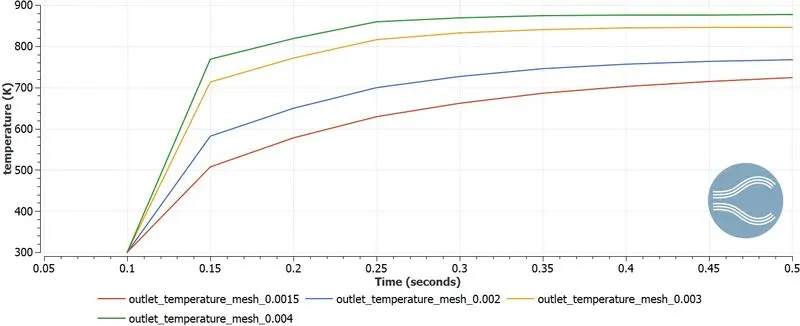
Above are the plots of mean temerature & temperature at outlet .From the plots we can see as ,we refine our grid size,the result accuracy increases and the temperature values converges to a perticular value for perticular grid size.Thus we will use refined grid to get accurate results.

MESH AT DEFFERENT GRID SIZES -

For Grid Size of 0.003 m

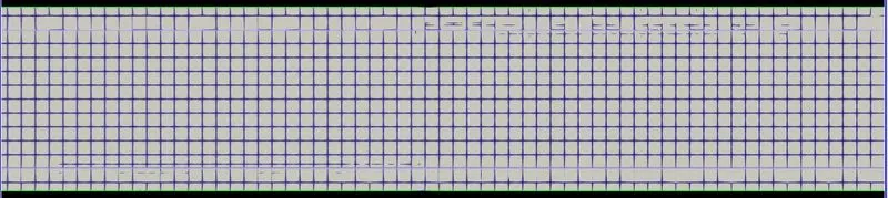
For Grid Size of 0.002 m

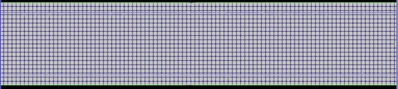
For Grid Size of 0.0015 m

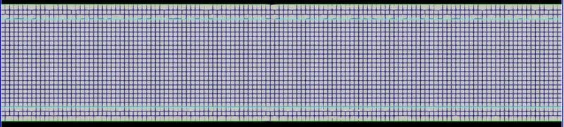
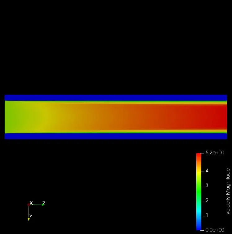
VELOCITY CONTOUR AT DIFFERENT GRID SIZES -

At 0.0015 m

At 0.002 m

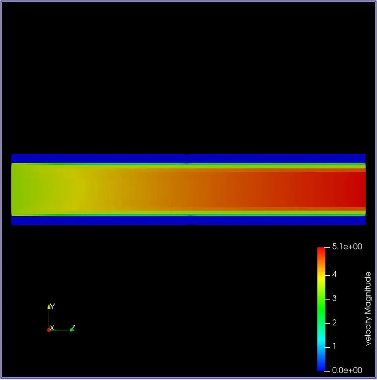
At 0.003 m

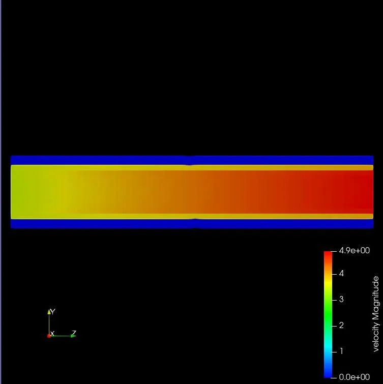
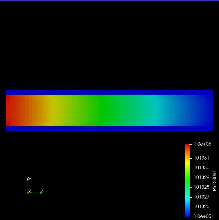
PRESSURE CONTOUR AT DIFFERENT GRID SIZES -

At 0.0015 m

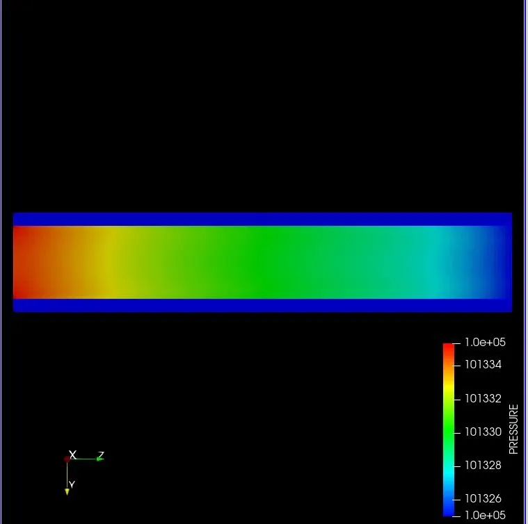
At 0.002 m

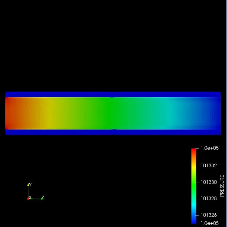
At 0.003 m

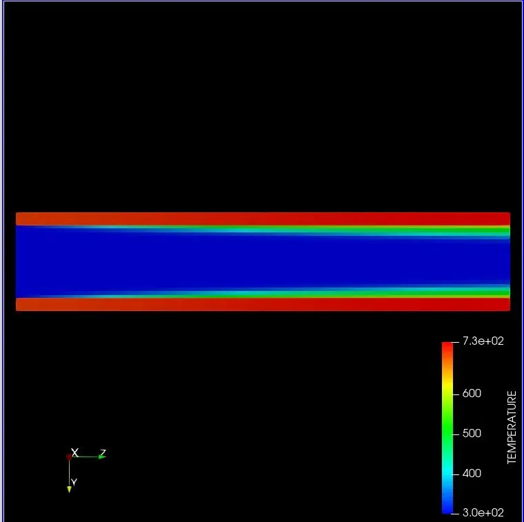
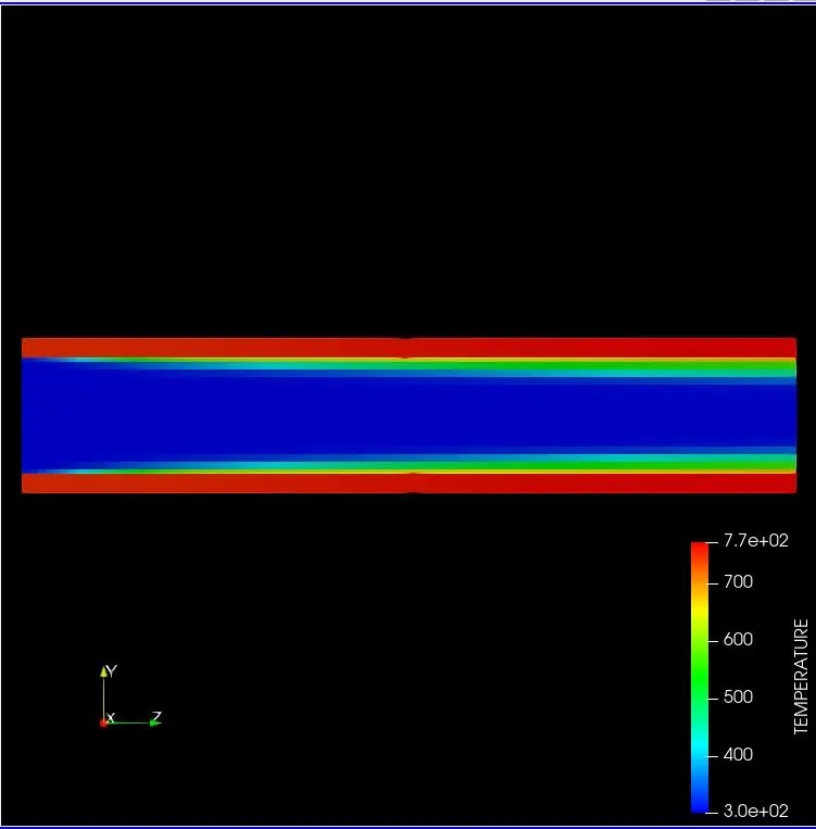
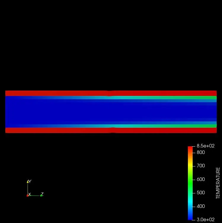
TEMPERATURE CONTOUR AT DIFFERENT GRID SIZES -

At 0.0015 m

At 0.002 m

At 0.003 m

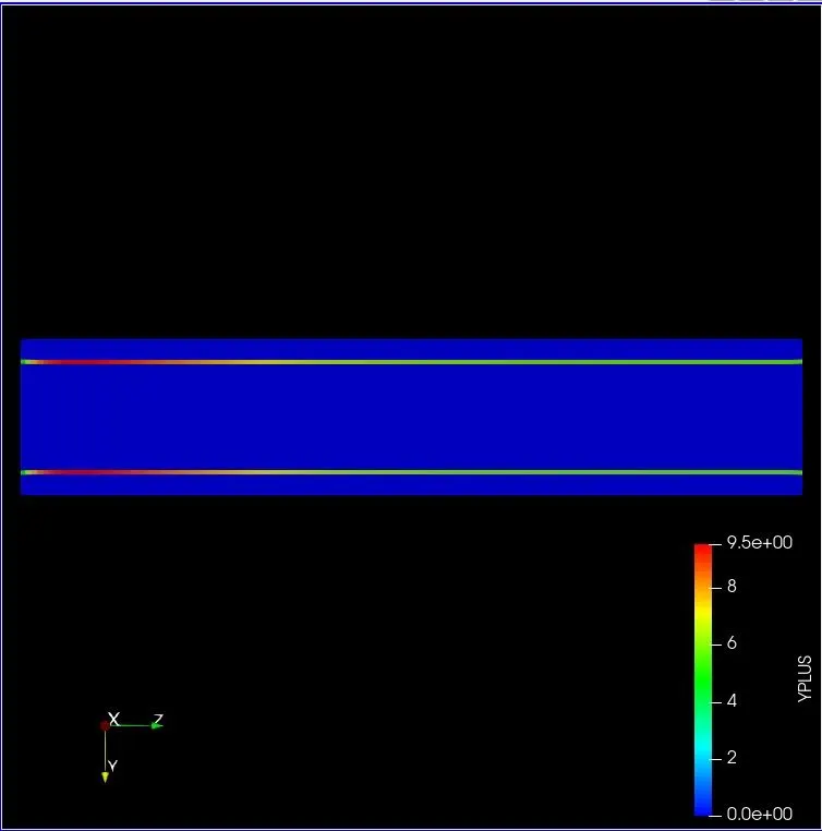
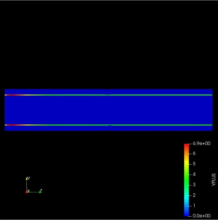
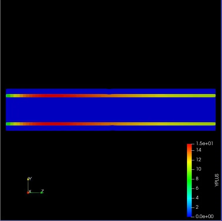
Y+ CONTOUR AT DIFFERENT GRID SIZES -

At 0.0015 m

At 0.002 m

At 0.003 m

EFFECT OF SUPER CYCLE STAGE INTERVAL -

To see the effect of supercycle stage interval on the on the total simulation time we will choose the mesh size of 0.004.

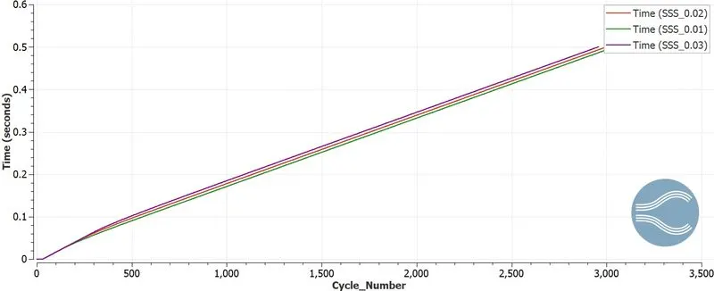
From the above plot it is clear that as the super cycle stage interval decreases ,simulation time increases.This is because there are more freezing of fluid side solver in order to solve solid side .

TOTAL CELL COUNT

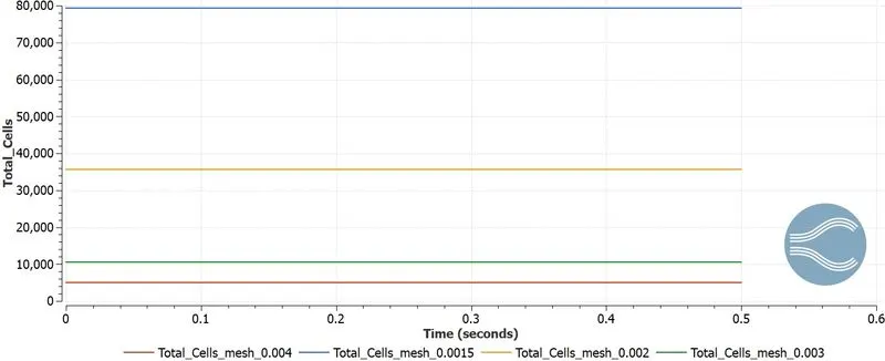
Grid Size	0.0015	0.002	0.003	0.004
Number of Cells	79264	35600	10496	5000

ANIMATIONS :

Temperature Animation at Grid Size of 0.0015 m

https://www.youtube.com/shorts/9gTh7u4JnEk

Temperature Animation at Grid Size of 0.002 m

https://www.youtube.com/shorts/mJogrodsayw

Temperature Animation at Grid Size of 0.003 m

https://www.youtube.com/shorts/rm9odKD_DzI

CONCLUSION :

*Supercycling overcomes the time scale disparity between fluid and solid regions.The lower supercycling interval results in higher computation time.

*Thus CHT analysis on a flow through pipe has been performed successfully.