Week 5 - Rayleigh Taylor Instability
Aim-
To study and perform Rayleigh Taylor instability simulation between two different fluid medium with different grid size and to
validate the results by Atwood number.
Objective -
*We are going to be learning volume of fluid(VOF) method,which is use to simulate two phase flows.
*Discuss some practical CFD models that have been based on the mathematical analysis of Rayleigh taylor waves and explain how these mathematical models have been adapted for CFD calculations.
*Perform Rayleigh Taylor instability simulation for air and water with 2 different mesh size,with the base mesh being 0.5 mm.
Compare the results by showing the animations.Observe the differences in the animation and explain the effects of mesh size on simualtion and also,explain why a steady state approach might not be suitable for these type of simulation.
*Then we will run one more simulation with water and user defined material(density = 400 kg/m^3,viscosity = 0.001 kg/ms)for refined mesh.
*Define the Atwood number and find out the Atwood number for both the cases and explain how the variation in Atwood number in the above two cases affects the behaviour of instability.
Introduction and Theory -
Rayleigh-Taylor(R-T) Instability : The Rayleigh Taylor instability occurs when a high density (`rho_1`) fluid is placed over a lower density (`rho_2`) fluid in a gravitational field.When the density interface is disturbed away from horizontal,the hydrostatic pressure acts to drive the heavier fluid into the lighter fluid,with disturbance amplitude growing exponentially,but shortly afterwards saturating and forming a characteristics mushroom shape,at least for some time.Eventually,either other wavelengths become important and accelerate the development of instability,or mixing or dilution of the density contrast will lead to a decelerration. Such naturally occuring R-T instabilities are quite common e.g.in oceans,supernovae and oil trapping salt domes.
There are four stages in Rayleigh Taylor instability -
Stage 1 -
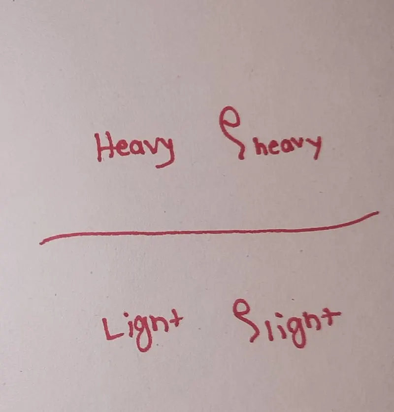
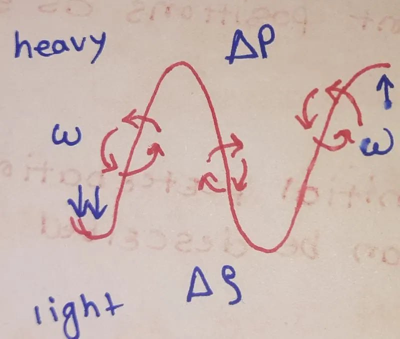
High density fluid on top and light density fluid at the bottom,because of this Rayleigh Taylor instability will occur and it will
cause small initial perturbations.
Because of different in densities,there will be difference in pressure at different positions as shown by the arrows.
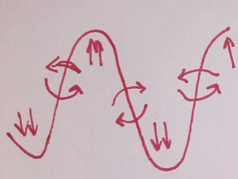
For calculation assum,initial perturbations to be in the form of cosine,which can be described by following formula,
`psi(x,t=0)` =`B_0cos(alpha*x)`
where,
`B_0` = Initial amplitude
`alpha` = special wave number
g = gravitational acceleration
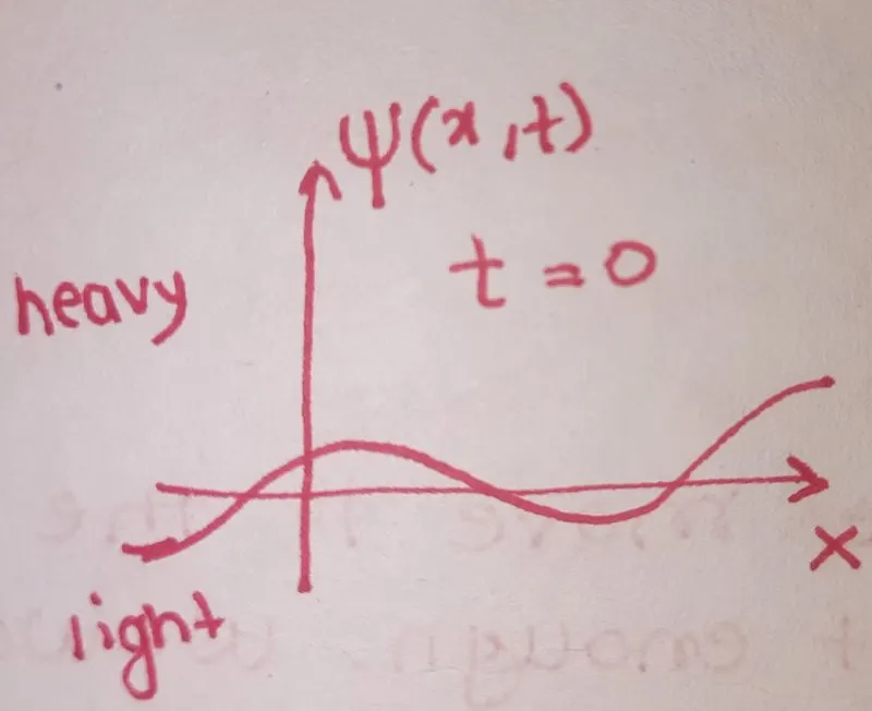
The initial amplitude grows at an exponential rate described by growth rate`gamma`,which is dependent on wave number `alpha`,
`psi(x,t)` = `B(t) cos(alpha*x)`
where,Amplitude B(t) =`B_0*e^(gammat`
Growth rate(`gamma`) = `sqrt( alpha*g*A)`
where A = Atwood Number .
Altogether the development of wave function can be described by the following formula,
`psi(x,t)`= `B_0 exp(sqrt((alpha*g)(rho1 - rho2)/(rho1 + rho2)) *t)cos(alpha*x)`
where, `rho_1` -Density of heavier fluid
`rho_2` -Density of lighter fluid
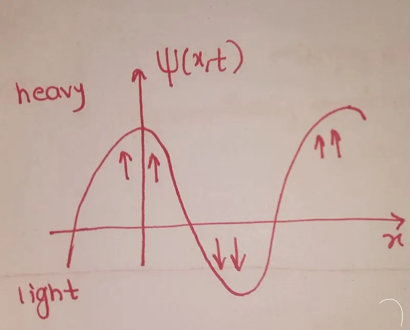
Another way to view the Rayleigh Taylor Instability is through the eyes of vorticity,
`vecw =vec nabla * vecu`
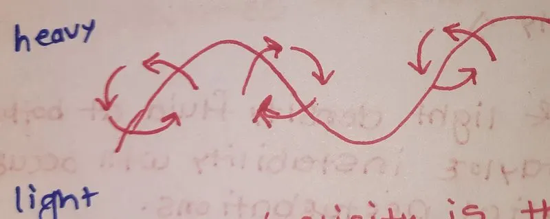
Vorticity is the rotation of the velocity of the fluid layers.The misalignment of density and pressure gradient in the two fluid
layers,will cause a torque at the interface which in turn creates vorticity.
Stage 2 -
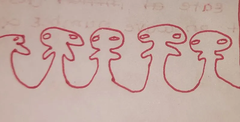
All the above discussion is good in 2D.But as we move to the second stage,the 2D description of the problem is not good enough.We would need to move to 3D spherical picture,to correctly describe the spikes and bubbles that form.
As can be seen in the picture ,spikes and bubbles form as instability continuous to grow.
Stage 3 -
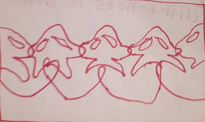
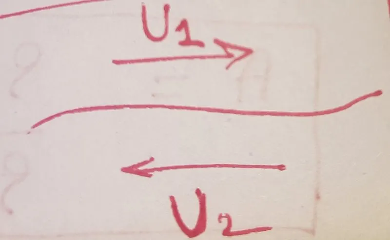
At this stage we encounter another instability,The Kelvin Helmholtz instability.This instability occurs when two fluids have
different velocities components,in direction parallel to interface as shown in below picture.
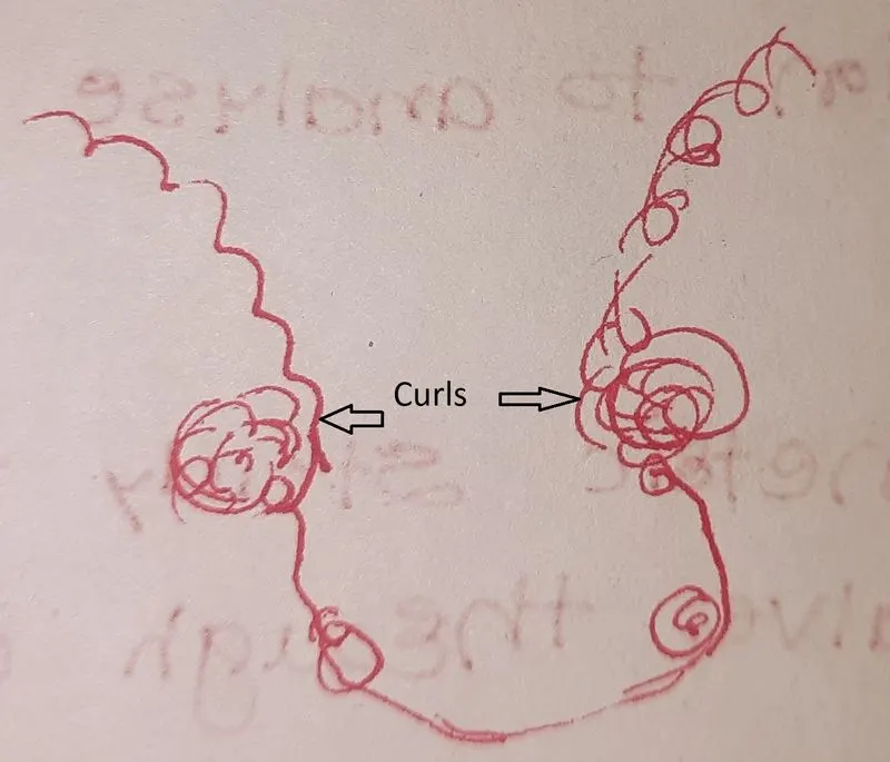
The Kelvin Helmholtz instability cause the spikes to form the characteristics curls around the mushroom clouds.
Stage 4 -
In the final stage the spikes will breakup and heavier fluid will dissolve into the ligher fluid in a chaotic way.
The RT instability is widely used in the CFD experiments in terms of several models and some of the widely used models are :-
1. Saffman-Taylor Instability
The Saffman-Taylor Instability occurs when a morphologically unstable fluids interfere in a porous medium.This is also called as viscous fingering.This type of instability can be seen in drainage,where a low viscosity fluid is pushed inside a pipe,where there is a fluid with higher viscosity.Most of the research using this model is done in the Hell-Shaw cells,boundary integral methods and phase field methods.
2. Richtmyer - Taylor Instability
The Richtmyer instability occurs when two fluids of different viscosity is impulsively accelerated.These effects can be seen in
shockwaves,where initially the shockwave is developed small and grows linearly with time.
3. Kelvin -Helmholtz Instability or Rayleigh Taylor Hybrid Model
This type of instability occurs when there is velocity shear in a continuous medium or when the velocity layer between two fluids are different.A classic example of this instability can be seen when atmospheric air blow over water.Also,this instability can be seen in Sun's corona,clouds and Saturn's bands.
4. Plateau -Rayleigh Instability
This instability model is used to explain how a falling water stream breaks into small droplets with same volume but with less
surface area.The fluid thread breaks up in fluid dynamics branch involves most of its study using the Plateau -Rayleigh Instability.
An example to demonstrate this effect is using the falling of water droplets from faucet/tap.When the faucet is closed or when the flow is interrupted,a long streaching of fluids occur at the neck of the faucet and if the faucet diameter is bigger,the fluid is not sucked back and breaks down into smaller water droplets.
5. Potential Flow Model
This model was developed by Layzer and it provide info on the movement of fluids in a circular tube.A constant supporting pressure(Atwood =1) is present,competition for both Rayleigh Taylor and the Richtmyer - Meshkov Instabilities.
Atwood Number -
In fluid dynamics Atwood number is used in the study of hydrodynamic instabilities in density stratified flows(i.e.to
characterize the density difference between two fluids).The Atwood number(A) is a dimensionless number
`A = (rho_1 - rho_2)/(rho_1 + rho_2)`
where, `rho_1` -Density of heavier fluid
`rho_2`-Density of lighter fluid
For big density differences A tends to 1.And for small differences A tends to zero.
Also with Atwood number the penetration distance can be defined by`A*g*t^2`
Effect of Atwood Number on instability -
If A is nearer to 1,R-T instability takes place in the form of fingers.
If A is nearer to 0,R-T instability takes place in the form of bubble like plumes.
Why Transient state simulation ?
A steady state approach was not used for the Rayleigh Taylor instability simulation because,the steady state approach is
independent on the time progressed and it would benefit us only if we are interested in the end results.But,in this study we have to observe the pattern of the instability wave formed from time to time ,from the starting time of the simulation.This could only be achieved once we use a transient simulation.Since it is a time marching solution,we expect more accuracy from transient simulation.
Modelling Approach -
We have dense fluid(in this case water) on top and lighter fluid(air) at the bottom and their interface is going to be unstable when gravity is present.
Solution Procedure -
For solving the RT instability analysis ,we will follow the below procedure :-
Geometry Creation --> Meshing --> Setup --> Solution & Post Processing.
Geometry Creation -
* Launch the Ansys workbench.First drag and drop the Fluid Flow(Fluent)model into project schematic and double click on geometry to launch the SpaceClaim.
*In spaceclaim,in sketch mode draw a 20 mm * 20mm rectangle.
*Use pull tool to create the surface.
*In structure window -> right click surface -> move to new component -> name it as air.
*Now we have to create another rectangular domain for water.Use same procedure as above & draw another rectangle on the top side of previous one.
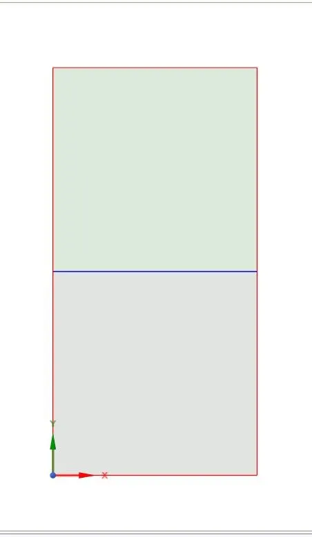
*Now when will do the meshing, we want our mesh to be conformal,for that we need share topology.
*click workbench -> share prep -> select both rectangles by draging box around them -> click share -> ok.
*This concludes our geometry preparation.Close ansys spaceclaim.
Meshing -
*Now,go to meshing, by double clickng on mesh in project schematic.
*First generate basic mesh with the element size of 0.5 mm.
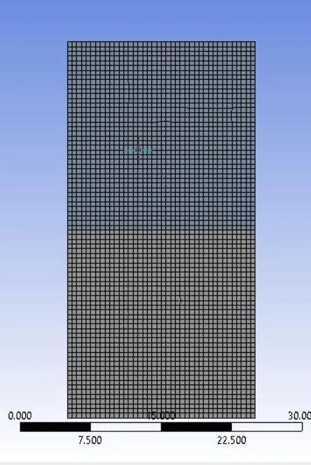
*Now we need to check our mesh quality.To do that in details of mesh ,go to quality => mesh metric => element quality.
*Here our minimum mesh quality is good enough.So now we can setup our problem.
*Close mesh and update the mesh.
Setup -
* Double click on setup in project schematic.This will open ansys fluent.
* Click on check mesh and make sure there are no errors.
* Our solution method will be SIMPLE,and will use pressure based solver.
* For momentum select second order upwind scheme & for pressure select PRESTO.For transient simualation first order implicit scheme is chosen.
* In this project we will run transient simulation,because we want to see how the interface collapses as a function of time.
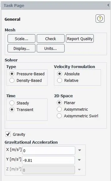
* We need to enable gravity.Since our geometry is in XY-plane,give negative value for acceleration due to gravity.
General => Gravity =>Gravitational acceleration => Y(m/s) = -9.81 `m/s`.
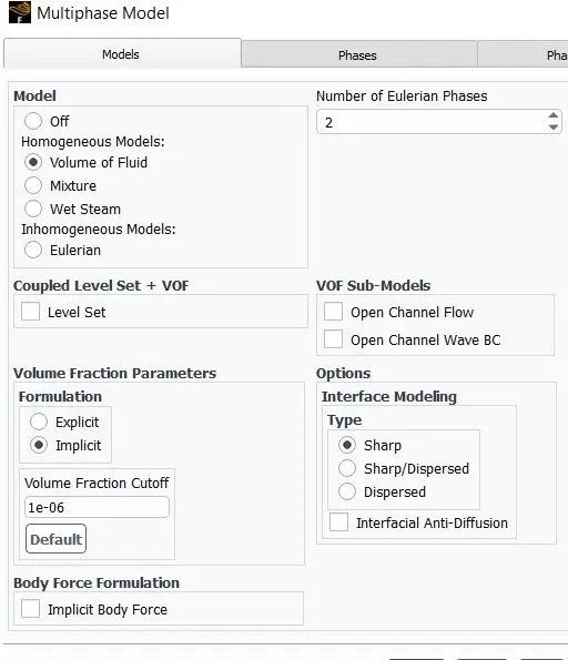
* Now we need to define number of eulerian phases and volume fraction parameters.To do that,
setting up physics => models => multiphase => in multiphase model => model => volume of fluid => Give number of eulerian phases = 2(one for water and one for air) and select volume fraction parameters as implicit => ok.
*Define the material as follows,
setting up physics => materials => click on fluent database => scroll down and select water-liquid(H_2O) => copy it and close both windows.
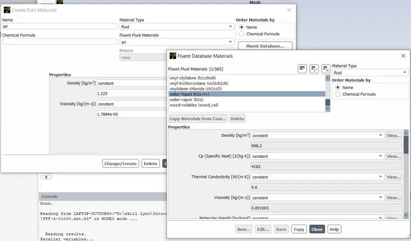
*Above we have decided number of materials and now we need to define which phases,
setting up physics => phases => click on list/show all =>select phase 1 primary phase and name it air,choose phase material air =>Now select phase 2 secondary phase,name it water and choose water as phase material.
*In our geometry we have two rectangles and we need to attach or patch our phase material to them,so that fluent knows which one is water and which one air.But before that we need to initialize our solution.
Solving => initialization => method standard => click on initialize.
*Now we can do the patching,
Solving => initialization => patch =>
1) First select phase as water & select volume fraction.=> in zones to patch select the water surface => give value 1 =>click on patch.
2) In zones to patch select the air surface => give value 0 =>click on patch => close window.
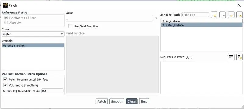
*In above steps we have assigned values for different patches,what does it mean ? Well we have two phases,the phases are represented by the value called alpha.If alpha = 1,it represents one phase,it could be water or air.And when alpha = 0, it represents other phase.
*Above for alpha = 1,we have water,which means when we initialize,we will get alpha= 1 , only at the top and alpha = 0 at the bottom.Then we ensure that our initialization process is correct.
*Now,how to,make sure that initialization is setup correctly,we need to plot contours,
go to post-processing => graphics => contours & select new => in contour of ,select phases => select water phase => select all surfaces => save/display.
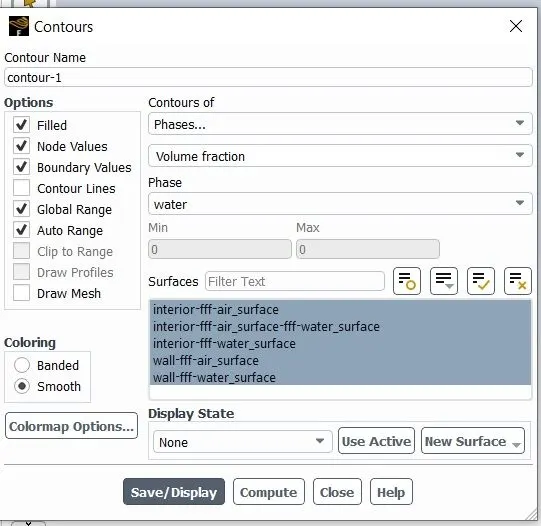
*We can see that volume fraction of water is 1 at top and 0 in the bottom.This confirms that our setup is correct.
*To create the animation go to solving => activities => create => solution animation => select the above created contour as animation object => preview the view and select the desired view => ok.
*Now run the calculation for 1000 time steps,with time step size being 0.005.If any error occurs try to change under relaxation factor or change the discretization scheme.
Post Processing and Results -
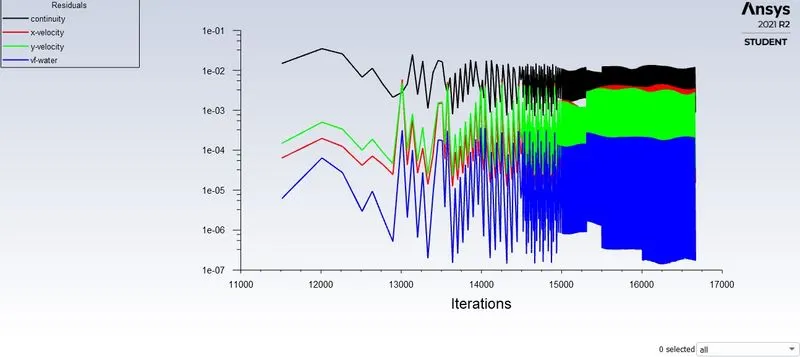
Residual Plot -
We can observe from the below residual plot that our solution has converged.
Volume Fraction of Water -
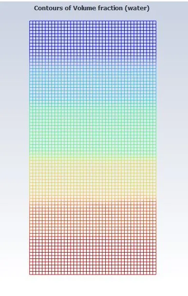
Animation of Rayleigh Taylor instability for coarse mesh -
https://drive.google.com/file/d/1-5vXthN6IjHKiUDAY-63J2FZ94sbafrB/view?usp=drivesdk
Case 2 - Fine mesh of size 0.1 mm
*Geometry procedure will be same.The only difference is in mesh ,change element size to 0.1 mm,generate mesh,close and update mesh.
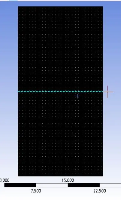
*Problem setup is almost same.But since the mesh is finer we need to run the simulation for more number of time steps than the previous one.
*Lets run the simualtion for 2000 time steps and time step size of 0.002 and go straight to post processing.
Post-Processing -
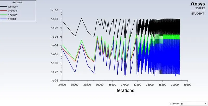
Residual Plot -
We can observe from the below residual plot that our solution has converged.
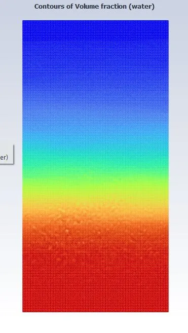
Volume Fraction of Water -
Animation of Rayleigh Taylor instability for fine mesh -
https://drive.google.com/file/d/1-6QdfCV2ktnfLKHxu2evBOdIufWhNpHE/view?usp=drivesdk
* Here we can observe volume fraction of the same problem with different mesh sizes.Finer the mesh gets,the accuracy of the results increases at expense of more computational effort,which we can observe from the above plots and solution animations.
*At the start,fluid behaves linearly,and we can observe small linearity sinking going on between them,slowly chunky bubbles from the higher density fluid on top settles down.This can be observed from the highest density mesh,resuting in the finest behaviour of instability.We can observe small linear perturbations at the start develops into more chaotic turbulent disturbances.Also a single globule transitions into multiple small globules.
*As the simulation progresses we can observe the formation of small mushroom bubbles,and as they rise we can see the formation of voticies along side them,which is also known as The Kelvin Helmholtz instability.This instability occurs when two fluids have different velocity components,in direction parallel to interface.
*As the simulation progresses amplitude of the perturbations increases,low density bubbles rise up and high density bubbles settles down.Also the thickness of the interface is smaller in finer mesh ,which results in better volume fraction conotur and results.
Case 3 - User Defined Material and Water,at mesh of size 0.1 mm
*Geometry & mesh procedure will be same as per case 2.Only difference is in the setup.Change the properties of lighter material which in this case is air.
setting up physics => materials => change density to `400 (kg)/m^3`& vicosity to 0.001 `(kg)/(ms).`
* Patch the material to appropriate side .
*Lets run the simualtion for 2700 time steps and time step size of 0.002 and go straight to post processing.
Post-Processing -
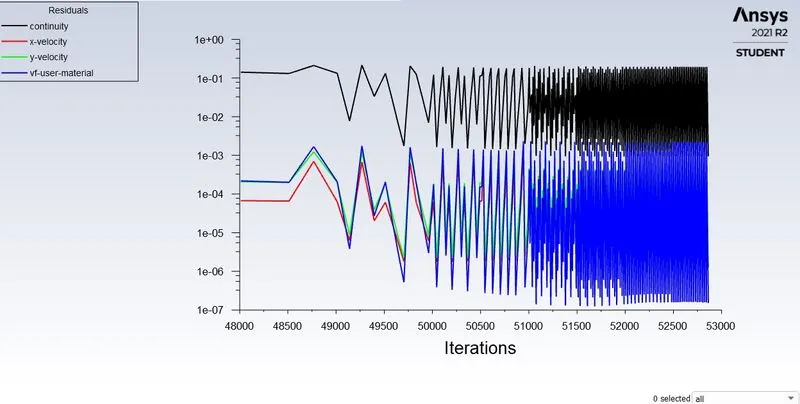
Residual Plot -
We can observe from the below residual plot that our solution has converged.
Volume Fraction of Water -
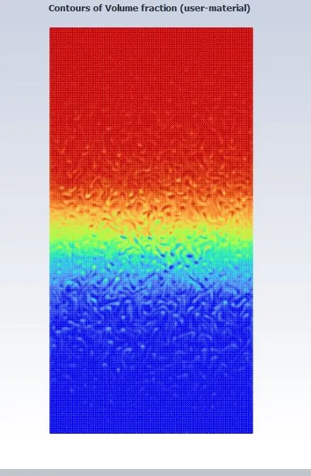
Animation of Rayleigh Taylor instability for user defined material with fine mesh -
https://drive.google.com/file/d/1-CcOVkfaepn-Zh-BYfGcjGDAIL0a_1IZ/view?usp=drivesdk
Atwood Number for above cases -
For Case 1(Air & Water) -
`(998.2-1.225)/(998.2+1.225) = 0.9975`
For Case 3(User Defined Material & Water) -
`(998.2-400)/(998.2+400) = 0.4278`
Effect of Atwood number on above 2 cases -
*As the Atwood number increases the evolution of interface grows faster,amplitude of perturbations increases i.e. larger the
Atwood number stronger is force at the interface to develop instability.
*In case 3,we could see there are spikes and bubbles formed ,where as in case 2 only sharp spikes formed when the instability takes place.
*From the results we can see that,when the Atwood number increases,there is increase in spike formation between two fluids as in case 2 and it decreases in case 3.Thus the results obtained from the simulation are validated by Atwood number calculation.
Conclusion -
*We performed the Rayleigh Taylor instability for two different cases & the numerical simulation is validated by Atwood Number.
*Transient solver better captures the flow compared to steady state but at the expense of computation time.
*Larger the Atwood number stromger is force at the interface to develop instability.