Week 9 - FVM Literature Review
Aim :-
To understand how Finite Volume Method (FVM) works,learn about the different types of schemes used in discretization and understand the function of flux limiters.
Introduction :-
Before learning about FVM, first we need to know,what do we expect from discretisation.Following are the 3 main expectations from a discretization method,
1) Conservativesness
2) Boundedness
3) Transportiveness
1) Conservativeness
If the physical problem involves the conservation of the variable,the discretize equation should also reflect
physicallythe same conservation.i.e.if you are having a collecton of discrete equations,alltogether sumed up,they should
represent the conservation of the physical variable over the entire control volume or over the entire domain.
This is not guaranteed from finite difference method (FDM).It is just a mathemattically expanded taylor series and
we never enforced any requirement of conservation.Conservativeness is not an inbuilt part of FDM.
2) Boundedness
Consider a rod ,whose one end is at 0 degree celcious and other end is at 100 degree celcious.There is no heat source.
And we are interested in the temperature distribution in this rod.So between these two points the temperature should be between 0 & 100.This is the physical description of the problem and discretization should also ensure this boundedness.
3) Transportiveness
If there is predominant direction of flow,then properties should be having a predominant transport direction based on
the flow direction.
For example,if flow is high reynolds number flow and any property say,enthalpy being transported.Then enthalpy will
predominantly transported along the direction of flow and not predominantly in opposite direction.
As fluid flow is governing the behaviour for high reynolds number,so transport direction should be in direction of
high reynolds number.This is transportiveness.
Finite Volume Method
The finite volume method is a method for representing and evaluating partial differential equations in the form of
algebraic equations.In the finite volume method ,volume integrals in a partial differential equation that contain a divergence term are converted to surface integrals,using the diergence theorem.These terms are then evaluated as fluxes at
the surfaces of each finite volume.
But to evaluate the integral,we need to know how flux varies between grid points.So when we consider a control
volume (CV),the CV should be represented by certan points.So we have centroid of the CV which is corresponding grid point.
In FVM the representative grid points are located at the geometric centers of the corresponding volumes.This is the convention in FVM,as it is mathematically much easier to handle with the centroid of the volume element,where we know,where it is located.
In FVM we have to represent values of flux at dixcrete grid points.So we require an interpolation function i.e. flux
as a function of position.As we choose interpolation function,then we can integrate it.After integration we get result as a
function of flux at the discrete grid points for each CV.
The reason for integration is that,when we are considering a differential equation,the differential equation(DE) is valid at a point,so when we integrate DE,it is now valid over a domain.In FVM we start with CV of differentiallly small size to derive the differential equation(DE),then we integrate the DE back on control volume of finite size,hence the name Finite Volume Method(FVM).
The main advantage of FVM is that, it carries the physical meaning of conservation with itself.When we integrate DE
over the domain,it imply that,we are now satisfying the conservation principle over the entire domain.
In FVM we use interpolation to evaluate integrals.And once the integrals are evaluated ,the history of iterpolation
is not important.This means we get freedom to choose different interpolation functions for different terms,as we don't
require those interpolations anymore for subsequent analysis.
The FVM's strength is that it only needs to do flux evaluation for the cell boundaries.This also holds for non linear
problems,which nakes it extra powerful for robust handling of (nonlinear)conservation laws appearing in transport problems.
The local accuracy of the FVM,such as close to a corner of interest,can be increased by refining the mesh around the corner.
However,the functions that approximate the solution whenusing the FVM cannot be easily made of higher order.This is the
disadvantage of FVM compared to FDM.
The basic advantage of FVm is ,it does not require the use of structured grids,and the effort to convert the given
mesh in to structured numerical grid internally is completely avoided.
Steps in FVM :-
1) Divide the domain into small number of finite sized sub domains(control volumes).Each sub domain is represented
by a finite number of grid points.
2) Integrate the governing differential equaton over each sub domain.
3) Consider interpolation for evaluating above integrals, to express the result in terms of algebric quantities at
the grid points.
Difference Between Finite-Difference Method(FDM) & Finite-Volume Method(FVM)
Finite-Difference Method: Advantages and Disadvantages
Int he finite-difference method it easy to increase the “element order” to get higher-order accuracy. If you can fit the simulation in a rectangular or box shaped geometry using a regular grid, efficient implementations are much easier than for finite-element and finite-volume methods. Regular grids are useful for large scale simulations on supercomputers often used in, meteorological, seismological, and astrophysical simulations.
With the finite-difference method, you may easily run into problems handling curved boundaries for the purpose of
defining the boundary conditions. Boundary conditions are needed to truncate the computational domain. They represent
communication with the surrounding world, which is the part that you do not want to be included in your simulation. If one
can overcome the boundary-condition problem on curved boundaries, the method gives very efficient and high-quality results.
For computations that need high accuracy, the extra effort in making boundary-fitted meshes and the associated
complications of such meshes for the implementation may be worth it. Examples include Formula 1 car computational fluid
dynamic (CFD) simulations and space-shuttle CFD simulations. The finite-difference method is more difficult to use for
handling material discontinuities. In addition, it does not lend itself to local grid refinement or anything similar to adaptive mesh refinement. This may be needed to resolve local rapid variations in solutions such as around a corner of a
complex shape.In FVM conservativesness in not guaranteed.
Finite-Volume Method: Advantages and Disadvantages
The finite-volume method’s strength is that it only needs to do flux evaluation for the cell boundaries. This also holds for nonlinear problems, which makes it extra powerful for robust handling of (nonlinear) conservation laws appearing
in transport problems.
The local accuracy of the finite-volume method, such as close to a corner of interest, can be increased by refining
the mesh around that corner, similar to the finite-element method. However, the functions that approximate the solution
when using the finite-volume method cannot be easily made of higher-order. This is a disadvantage of the finite-volume method compared to the finite-element and finite-difference methods.
Need of Interpolation Schemes :-
Unlike the finite difference method,in finite volume method,the integral form of the governing equations are solved
considering an arbitary volume with central point P,about which the properties in the control volume are averaged.In
integrating the governing equation about the control volume,the limits for the intigral are the faces which istersect with
the adjacent control volume.In such a case,we need to determine the properties at points other than the mesh grid points.i.e.The approximation of surface and volume integrals require values of the variables at locatiions other than the computational nodes of control volume.Values at these locations are obtained using interpolation formulae.
Interpolation Methods :
Upwind Interpolation(UDS)
Linear Interpolation or Central Difference Scheme(CDS)
Quadratic Upwind Interpolation for Convective Kinematics(QUICK)
Hybrid and TVD Interpolation Schemes
Upwind Interpolation(UDS): Depending on the direction of flow the upwind interpolation scheme is equivalent to
calculating either the forward difference or the backward finite difference approximation. It is first-order accurate.
Linear Interpolation or Central Difference Scheme(CDS): Approximate values of the variable at the control volume face
centre by the linear interpolation of the values at the two nearest computational nodes. This scheme is equivalent to
using the central difference scheme. This interpolation is second-order accurate and may produce oscillatory solutions.
Quadratic Upwind Interpolation for Convective Kinematics(QUICK): The quadratic upwind interpolation scheme is derived using polynomial fitting. This is third-order accurate but prone to oscillations.It uses one downstream and two upstream points for computation.It has better damping properties in the solution than CDS.
Quadratic - As it uses 3 nodes.
Upwind - As it uses two upstreams.
Convective Kinematics - As it is used for convective domain problems.
Hybrid Interpolation: It is the blend of Upwind Interpolation(UDS) and Linear Interpolation or Central Difference Scheme(CDS).The hybrid difference scheme exploits the favourable properties of the upwind and central differencing schemes.It switches to upwind differencing when central differencing produces inaccurate results at high Pe numbers.The scheme is fully conservative and since the coefficients are always positive it is unconditionally bounded. It satisfies the
transportiveness requirement by using an upwind formulation for large values of Peclet number.
Total variation diminishing scheme (TVD): The fact that the QUICK scheme and other higher-order schemes can give undershoots and overshoots has led to the development of second-order schemes that avoid these problems. The class of TVD (total variation diminishing) schemes has been specially formulated to achieve oscillation-free solutions and has proved to be useful in CFD calculations.TVD schemes are designed to address this undesirable oscillatory behaviour of higher-order
schemes. In TVD schemes the tendency towards oscillation is counteracted by adding an artificial diffusion fragment or by
adding a weighting towards upstream contribution.
It is 2nd order accurate.
`f_e=f_p+1/2ψ(r)(f_E − f_P)`
where,
ψ(r) is called a flux limiter function
where,
`r = (u_i-u_(i-1))/(u_(i+1)-u_i)`
Flux Limiters:-
The idea of the flux limiter is to address the source of the oscillation.Interpolation is the source of oscillation.
Whenever we interpolate we either undershoot or overshoot.The way to deal with these oscillations is to figure out a way to
interpolate that does not create any new maximums or minimums.This scheme is call TVD.The reason it is call TVD ,has to do
with the enforcement of no new minimums and no new maximums.Bcause mathematically ou can prove that if you don't creat any new maximums or minimums also known as total variation,the spatial derivative is always a decreasing function.
For convective fluid flow, it is observed that low order schemes are usually stable but quite dissipative in nature
around the points of discontinuity or shocks while the higher order schemes are unstable in nature and show oscillations in
the vicinity of dinscontinuity or shocks. Highly accurate and oscillation free schemes are known as High Resolution Schemes.
In order to make the scheme TVD, we must constrain or limit the range of possible values of the additional convective flux
`f_e=f_p+1/2ψ(r)(f_E − f_P)`, which was originally introduced to make the scheme higher-order. Hence, the function `ψ(r)`
is called a flux limiter function.
Flux Limiter functions are used to fine tune the higher order and lower order schemes in such a way that the resulting scheme
gives a higher order accuracy in the smooth region of the flow and maintains first order accuracy in the vicinity of shocks
and discontinuities. For such a scheme TVD scheme is employed.
`F(u_(i+1/2)) = f^(low)(i+1/2) - ψ(r_i)(f^(low)(i+1/2)-f^(high)(i+1/2))`
`F(u_(i-1/2)) = f^(low)(i-1/2)- ψ(r_i-1)(f^(low)(i-1/2)-f^(high)(i-1/2))`
where,
`f^(low)` is low precision flux (first order)
`f^(high)` is high precision flux (higher order)
1D Steady State Heat Conduction with Heat Source
Now to understand Finite Volume Method (FVM) and to understand the above discussion better ,lets,consider 1D Steady
State Heat Conduction with Heat Source.
`d/dx(K(dT)/dx)+s=0`
Let's have a domain and divide it into subdomain or control volume(CV) as shown below -
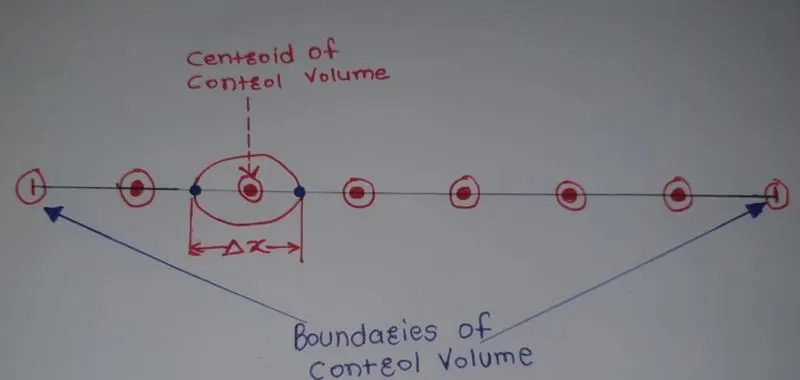
As each CV should be associated with the grid point,so we have centroid of each CV as shown in above figure.Also we require
boundaries of the CV through which we impliment boundary conditions.
Now lets isolate the control volume from the above figure and we will describe the features of the control volume,
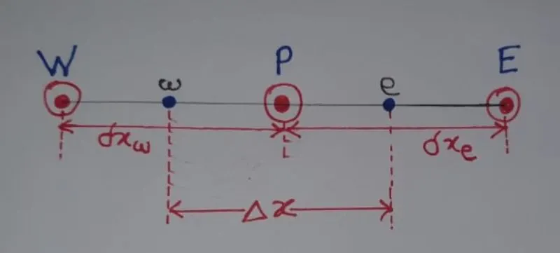
In above figure,
W - West side centroid
E - East side centroid
e - east face
w - west face
Integrate governinig differential equation over control volume,
`int_w^ed/dx(K(dT)/dx)dx+int_w^esdx=0`
`[(K(dT)/dx)]_e-[(K(dT)/dx)]_w+S(x_e-x_w)=0`
`[(K(dT)/dx)]_e-[(K(dT)/dx)]_w+SDeltax=0` -------------------eq.1
As T is linear function of x,therefore`(T_2-T_1)/(x_2-x_1)`
Therefore,
`[(K(dT)/dx)]_e = K_e(T_E-T_p)/(deltax_e`
Also,
`[(K(dT)/dx)]_w = K_w(T_P-T_W)/(deltax_w`
Where,
`deltax_e =x_e-x_P`
`deltax_w =x_P-x_w`
Hence,eq.1 becomes
`K_e [(T_E-T_P)/(deltax_e)]-K_w[(T_P-T_W)/(deltax_w)] + SDeltax=0`
`(K_e/(deltax_e)+K_w/(deltax_w))T_P=K_e/(deltax_e)T_E+K_w/(deltax_w)T_W+SDeltax`
We can sumbolically write it in the following way,
`a_PT_P=a_ET_E+a_WT_W+b` ----------eq.2
where,
`a_E=K_e/(deltax_e );a_W=K_w/(deltax_w) ;a_P=a_E+a_W ;b=SDeltax`
This is the finite volume discretize equation.
We can also write eq.2 interms of indices as,
`a_iT_i=a_((i+1))T_((i+1))+a_((i-1))T_((i-1))+b`
Where,
`P=i;E=i+1;W=i-1`
So,value of variable at one grid perticular grid point is expressed as,a function of values at it's neighbouring grid point,through algebric equation.
Conclusion:-
FVM is really a powerful approach to solve the CFD problems.With the help of proper interpolation scheme and accurate use of flux limiters in case any discontinuities present,we can solve a wide range of CFD problems.