Week 6 - CHT Analysis on a Graphics card
1] Aim -
To perform a steady state conjugate heat transfer(CHT) analysis on a model of a graphics card.
2] Objective -
*Perform CHT analysis on a Graphics card model by choosing appropriate material of choice.
*Give a brief description of where and why CHT analysis is used
*Find the maximum temperature & heat transfer coefficient attained by processor & also find the potential hot spots after simulation.
*Then vary the velocity from 1 m/s to 3 m/s and 5 m/s and compare the results.
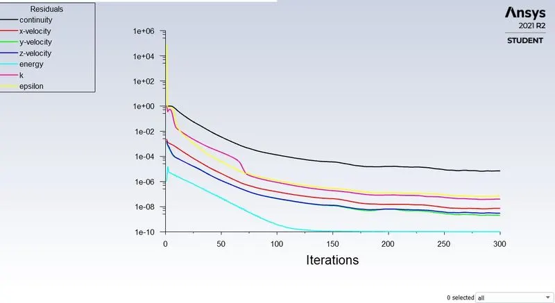
*Prove that simulation has converged using quality material which can show that solution has converged.
3] Introduction & Theory -
In this project,a steady state conjugate heat transfer analysis on a graphics card model is done.Graphic card has became an everyday used object and is a very important part of the computer system.This product is mass produced daily and has made computers exceptionally efficient.
A graphics card generates output images to a display device.Graphic cards generates heat as they compute numerical data while in use.So dessipating heat is very much essential in accordance with the performance.There are many cooling solutions which are provided by manufacturers,one of which is cooling fins.To dissipate heat more quickly ,wee need to increase the heat transfer coefficient around the fins.
3.1] Conjugate Heat Transfer (CHT) Analysis -
CHT analysis allows for the simulation of heat transfer between solid and fluid domains by exchanging thermal energy at the interfaces between them and transported via conduction within solids and aditionally via convection within fluid domains.
CHT analysis is beneficial in enigineering applications because it shows the heat exchanging capabilities between two surfaces
in the engineering device and various optimization can be done to improve the thermal characteristics of the devices.Thus,this can be used to improve the heat transfer rate wherever required.It also helps us to identify the key parameters to enhance the fluid flow and heat transfer within the system.
CHT corresponds with the combination of heat transfer in solid and fluid.In solids conductions dominates while in fluids
convection dominates.Efficiently combining heat transfer in fluids and solids is the key to designing effective coolers,
heaters or heat exchangers.The forced convection is the most common way to achieve high heat transger rate.In some applications performance is further improved by combining convection with phase change.CHT can be performed to improve the cooling performance of water jackets and increase the engine life.
There are three main modes of heat transfer -
*Conduction is the heat transfer that occurs when a temperature difference eists across a stationary medium.
*Convection is the heat transfer between a surface and a moving fluid when there is a temperature difference between the two.
*Radiation is the emission of energy in the form of electromagnetic waves.In the absence of an intervening medium,there is net heat transfer by radiation between two surfaces at different temperatures.
4] Modelling Approach -
CHT analysis is done on a graphic card model by applying heat on the processor of the graphic card ,while it contained in an enclosure.
The air is passed at a certain velocity through the enclosure and we observe the heat dissipation through the fins by conduction from the processor,then observe how the flowing air cools the fin and observe the heat transfer taking place through it.
5] Solution Procedure -
For solving the CHT analysis on a graphic card ,we will follow the below procedure :-
Geometry Creation --> Meshing --> Setup --> Solution & Post Processing
5.1] Geometry Creation -
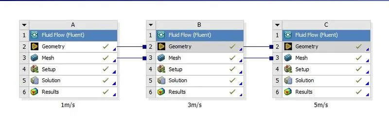
* Launch the Ansys workbench.First drag and drop the Fluid Flow(Fluent)model into project schematic and double click on geometry to launch the SpaceClaim.
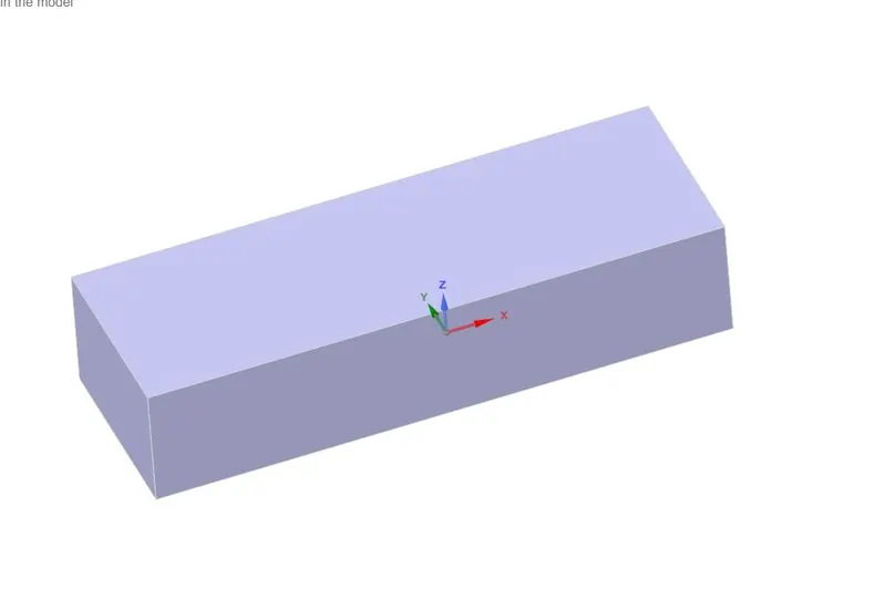
* Import the geometry into the ansys spaceclaim.The graphic card model used in this project is shown below,which is closed in an enclosure.
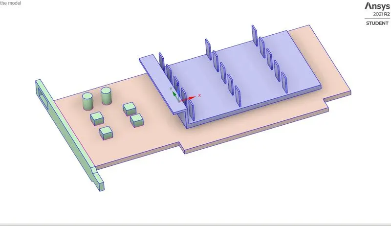
* Before going into meshing we need to make sure that the mesh which we will generate is a conformal mesh.
* Conformal mesh means the vertex of solid volume should be connected to the vertex of the fluid volume and perticular face of the fluid volume should be connected to the respective face of the solid volume.
* Now we need to enable share topology in ansys spaceclaim to achieve conformal mesh.
click workbench => share prep.
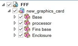
*Once we done this ,we will see pink and blue lines at the interface,that basically tells us where the things are being shared.
*Close the spaceClaim.
5.2] Meshing -
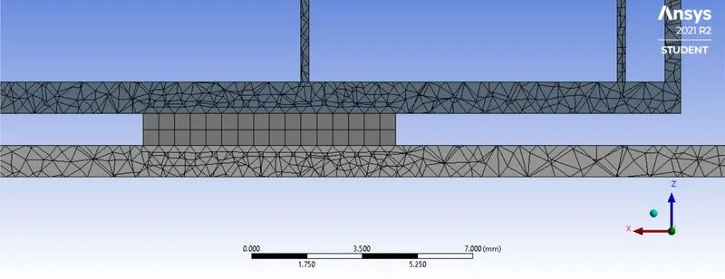
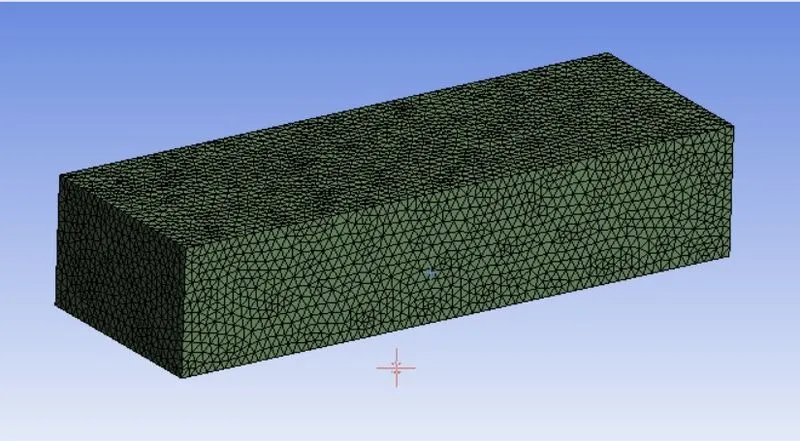
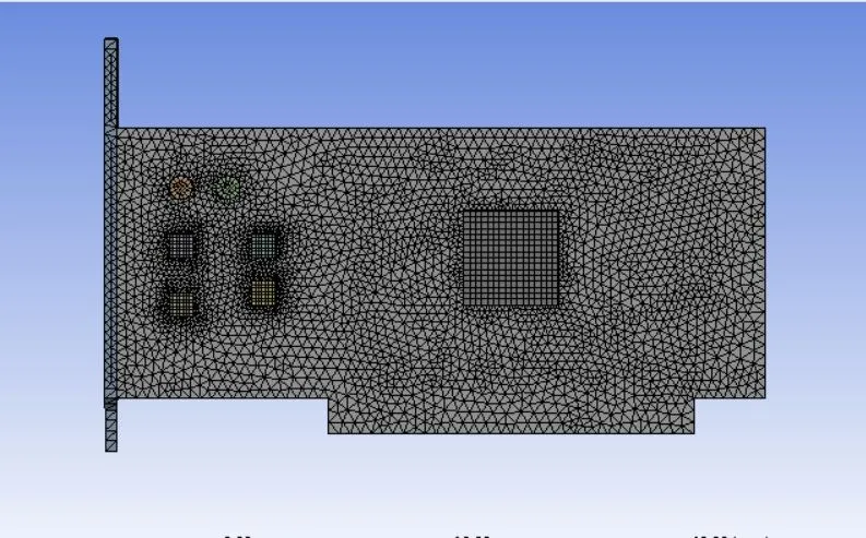
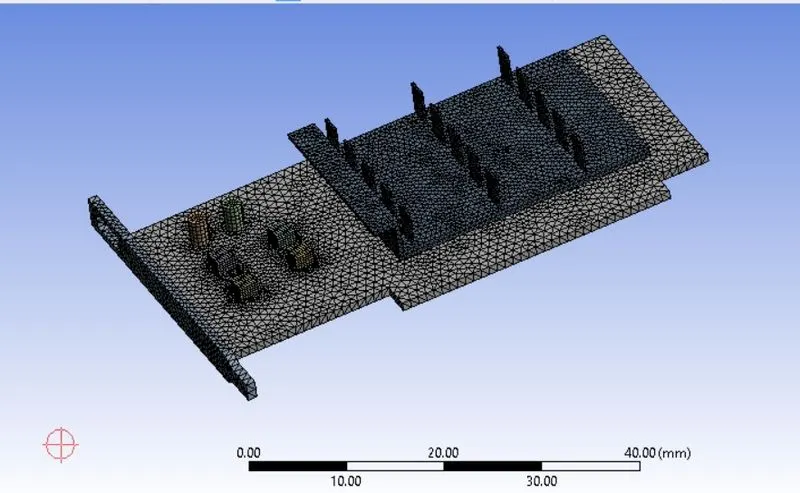
*Now,go to meshing, by double clicking on mesh,and first do the name selection i.e give proper boundary names.Then generate the basic mesh using generate mesh command.We can see the flow of the mesh inside the extracted volume by using section plane.Also we can check the mesh quality by using mesh quality option.
select the prefered body => press N => name the selection.
In meshing we can see the mesh is perfect.This is exactly how we need to make meshes for CHT cases.Always create the named selection first before generating the mesh.Select the edge you want to name,click N & name the selection.
*Then,next thing to do is to mesh.We click the mesh option in the side window and create our base line mesh.We then refine mesh.
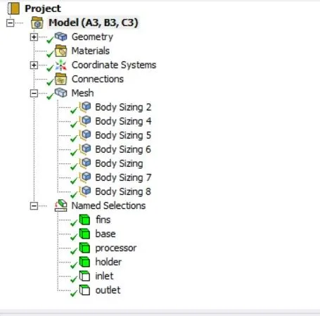
Processor body sizing -
*As processor is our main source of heat generation,to capture detailed heat distribution we need to refine the mesh on processor.
Right click mesh => sizing => in geometry select processor & give size of 0.5 mm => generate mesh.
Capacitor body sizing -
*Since capacitor contains round edges ,we need to capture them perfectly.
1] Right click mesh => sizing => in geometry select select cylindrical capacitors & give size of 0.2 mm => select yes for curvature capture => generate mesh.
2] Right click mesh => sizing => in geometry select select rectangular capacitors & give size of 0.3 mm => select yes for curvature capture => generate mesh.
Fins body sizing -
*Fins will be the main body which will distribute heat generated by the processor to the surrounding air via convection.Hence it also needs to be refined.
Right click mesh => sizing => in geometry select the fins & give size of 0.6 mm => generate mesh.
Enclosure sizing -
As enclosure isn't in direct contact with the processor we can set slightly coarser mesh for it.
*Now we will refine the enclosure,by giving global mesh size of 3 mm.
Base body sizing -
Also need to moniter conduction in base ,since the processor is soldered on it,so will refine it also.
Right click mesh => sizing => in geometry select the base & give size of 1 mm => generate mesh.
Holder body sizing -
At holder the max.heat transfer will be due to convection,so need to moniter it.
Right click mesh => sizing => in geometry select the holder & give size of 0.78 mm => generate mesh.
* Now lets check our mesh quality.Our minimum mesh quality is good enough.
* This concludes our meshing procedure.
* Now close the mesh & update.
5.3] Setup -
* Double click setup in project schematic.This will open ansys fluent.
*Click on check mesh and make sure there are no errors.
Setting up Physics
Our solution method will be SIMPLE.
We need to enable energy to capture temperature.
General -
*Solver type - pressure based
*time - Steady state
*velocity formulation - absolute
Models -
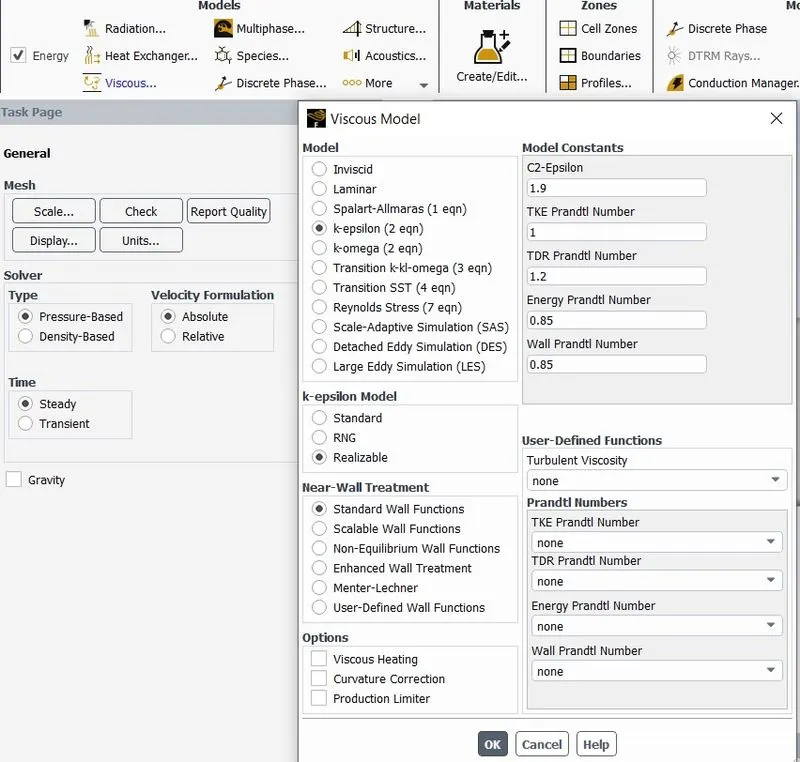
*viscous model - k-epsilon realizable
Material -
*Fluid - Air
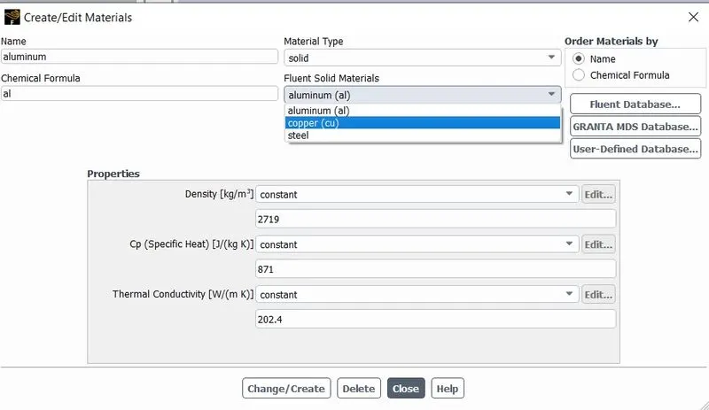
*Solid - Aluminum for fins,copper for processor and steel for all other components.
Zones -
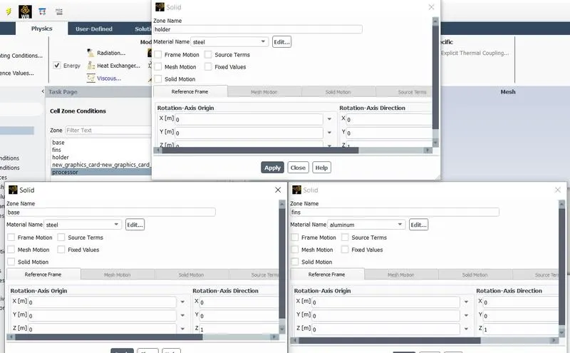
*In cell zones you will see fluid volume set to type fluid and in solid volume all the named selection are listed.Select aluminum as material for fins,copper for processor,and steel for all other components.
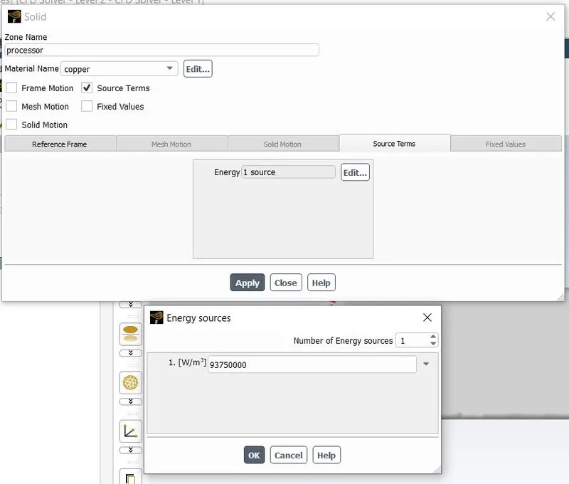
*For processor we will give internal heat generation as source term,we won't give it boundary conditions because,if we give there it will be constant around the whole domain and when you give it in the cell zone ,it will be given or generated at the center and spread around the whole processor.
Volumetric heat generated by the processor -
*Consider the power consumed by the processor is 6 W.
Volume of core is 64 mm(64*10^-9 m).
Heat flux density is the heat flux per unit volume ,which is our input for processor .
Heat flux density = source term = power/volume = 93750000 w/m^3
Boundary conditions - We can see all the named selections which,we generated above being used as boundary conditions.
* Inlet -
Type - velocity inlet
velocity magnitude - 1 m/sec
Initial Temperature - 300 k
* Outlet -
Type - pressure outlet
gauge pressure - 0 Pa
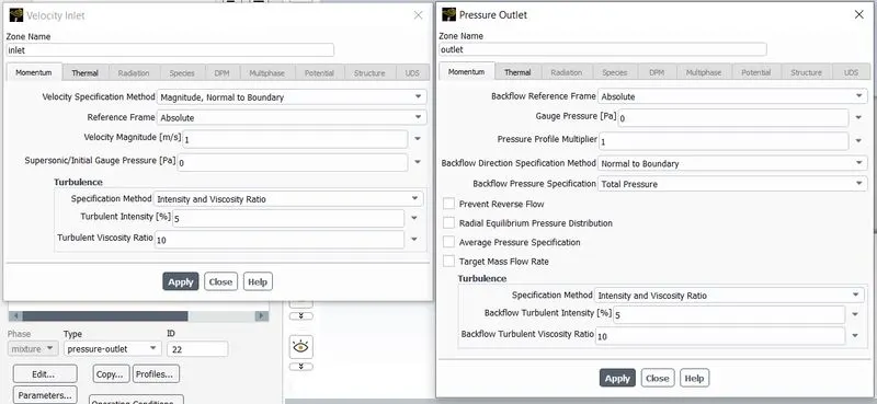
*Also we will check other boundary conditions,to make sure they are wall type and coupled(to couple the two sides of the wall).
*Now initialize the domain.We will use hybrid initialization,this provides very good initial conditions.
*We want to moniter different flow quantities as the solution is being generated,will use contours for this.We want to see how
the velocity & temperature variation looks like.
For temperature go to postProcessing => contours => new => contour of => Temperature => under it static temperature => select all the walls(all parts of graphic card)
& hit save/display.Simillarly create contour for velocity.
*To create animation,go to activities => solution animation => select temperature contour => preview => set desired view => give name as temperature animation.
6] Solution & Post Processing -
Case 1 => 1 m/s
Residual Plot -
*We can see that solution has converged after about 275 iterations.
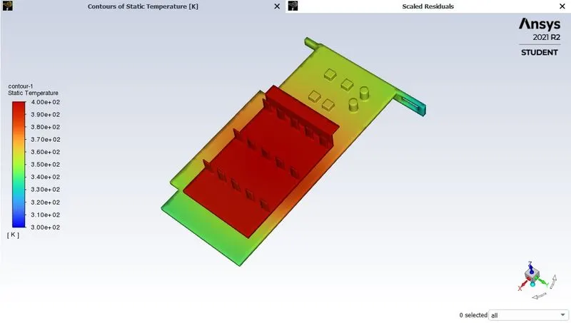
Temperature Contour -
*Below is the plot for temperature contour.It can be observed that,high temperature regions around processor, which is mainly due to conduction
Heat Transfer Coefficient Contour -
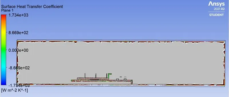
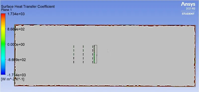
*Below is the plot for heat transfer coefficient contour on graphic card.We can see that maximum heat transfer due to convection is at the capacitors,which is mainly due to their shape,as heat transfer depends on area.It increases as the air velocity increases.
*Also as the fluid stream passes over the fins,intermixing takes palce and heat transfer increases.
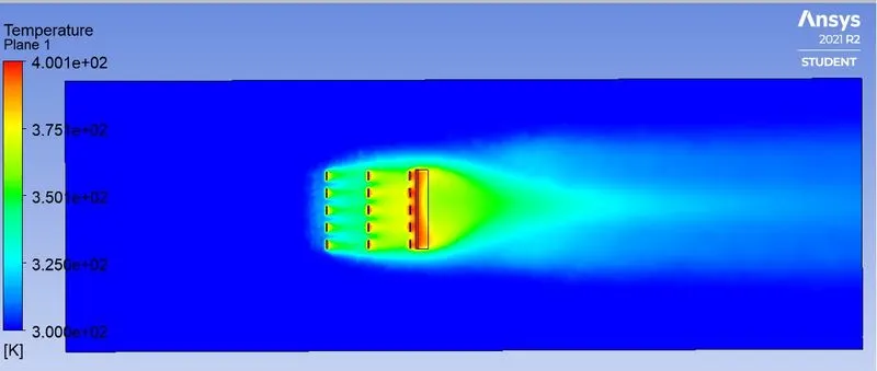
Plane Temperature Contour -
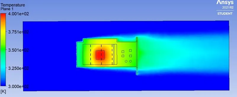
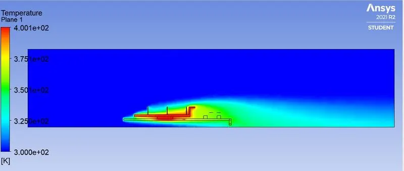
*Below is the plot for temperature contour on plane.It can be observed that,high temperature is at the end of the fins,this is mainly due to recirculation region.We can observe this clearly in velocity contour.
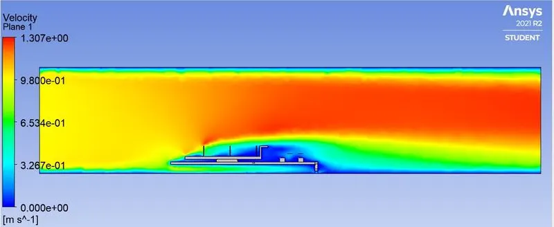
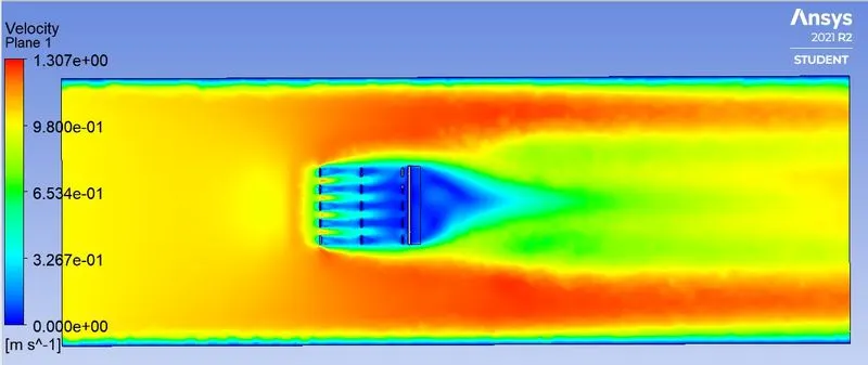
Plane velocity contour -
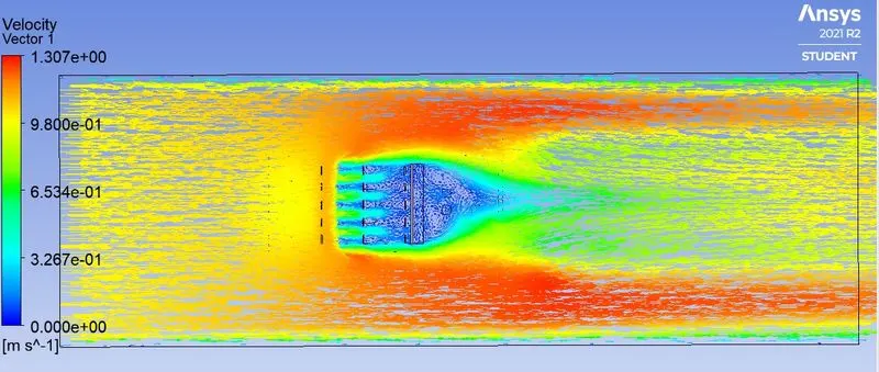
*In the below contour plot we can see that,velocity at the end of the fins is almost close to zero because of recirculation
region.The recirculation region can be visualized clearly in vector contour plot.
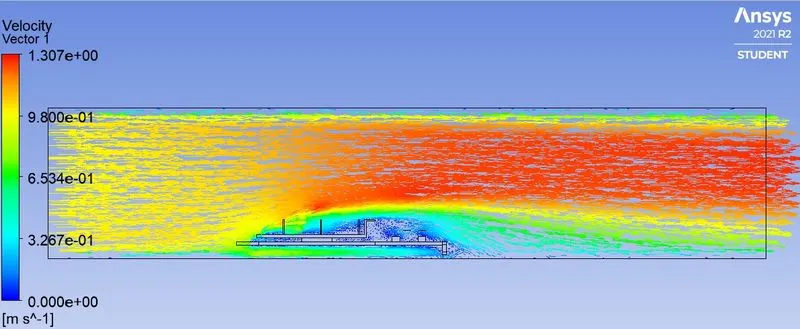
Plane velocity vector contour plot -
In the below plot velocity vectors are plotted on mid plane ,while temperature is plotted on midplane and graphic card.It
can be observed that,the places where temperature is high,is also the region of recirculation.
Case 2 => 3 m/s
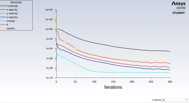
Residual Plot -
*We can see that solution has converged after about 275 iterations.
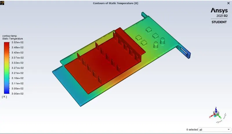
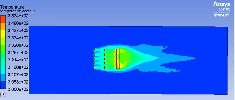
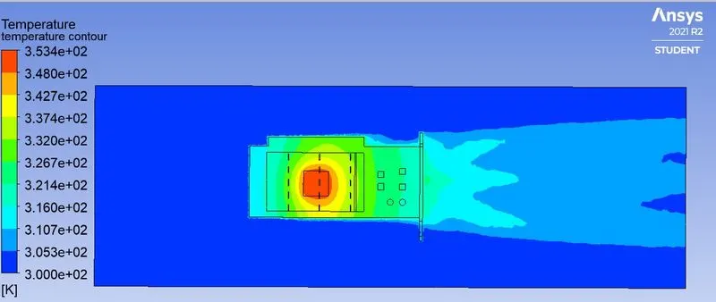
Temperature Contour -
*Below is the plot for temperature contour.It can be observed that,high temperature regions around processor, which is mainly due to conduction
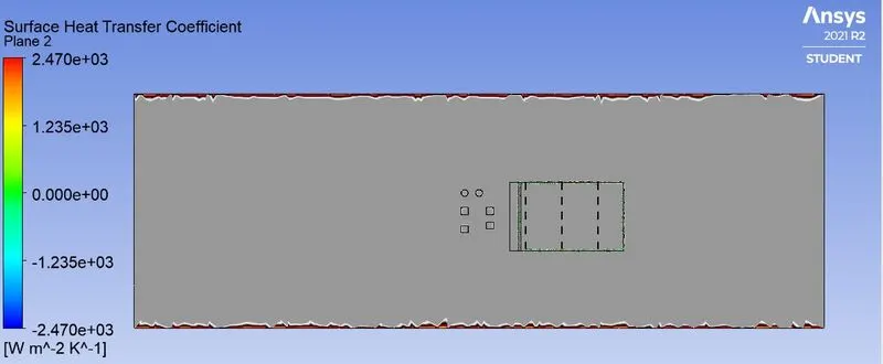
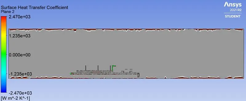
Heat Transfer Coefficient Contour -
*Below is the plot for heat transfer coefficient contour on graphic card.We can see that maximum heat transfer due to convection is at the capacitors,which is mainly due to their shape,as heat transfer depends on area.It increases as the air velocity increases.
*Also as the fluid stream passes over the fins,intermixing takes palce and heat transfer increases.
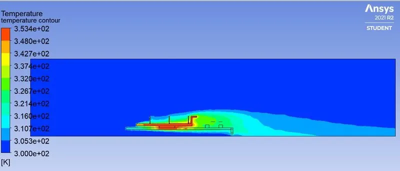
Plane Temperature Contour -
*Below is the plot for temperature contour on plane.It can be observed that,high temperature is at the end of the fins,this is mainly due to recirculation region.We can observe this clearly in velocity contour.
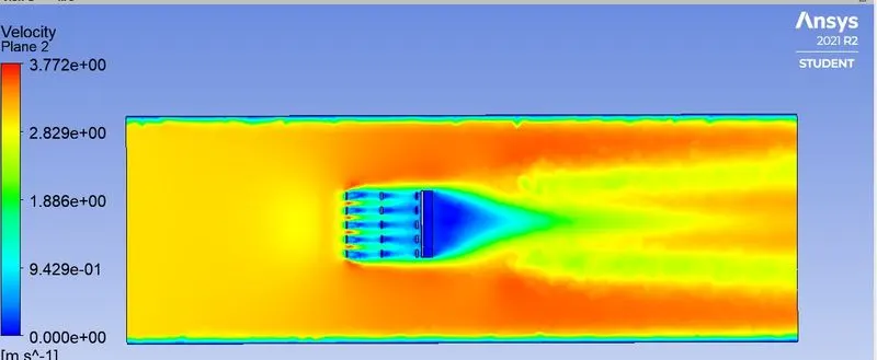
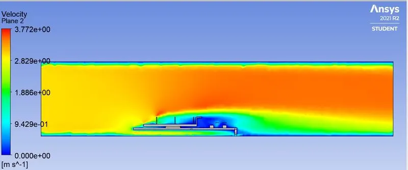
Plane velocity contour -
*In the below contour plot we can see that,velocity at the end of the fins is almost close to zero because of recirculation
region.The recirculation region can be visualized clearly in vector contour plot.
Plane velocity vector contour plot -
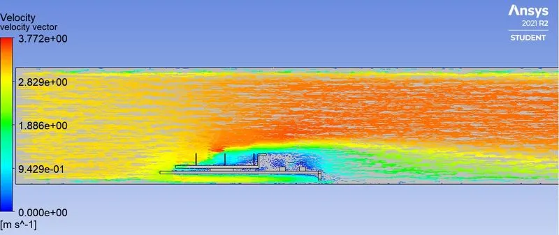
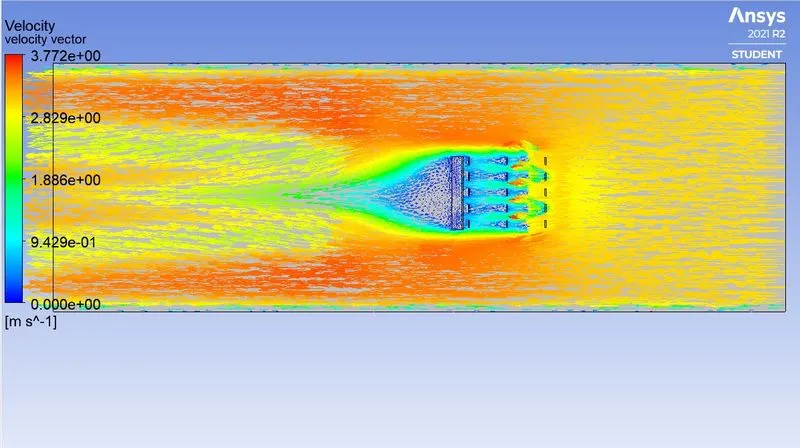
In the below plot velocity vectors are plotted on mid plane ,while temperature is plotted on midplane and graphic card.It
can be observed that,the places where temperature is high,is also the region of recirculation.
Case 3 => 5 m/s
Residual Plot -
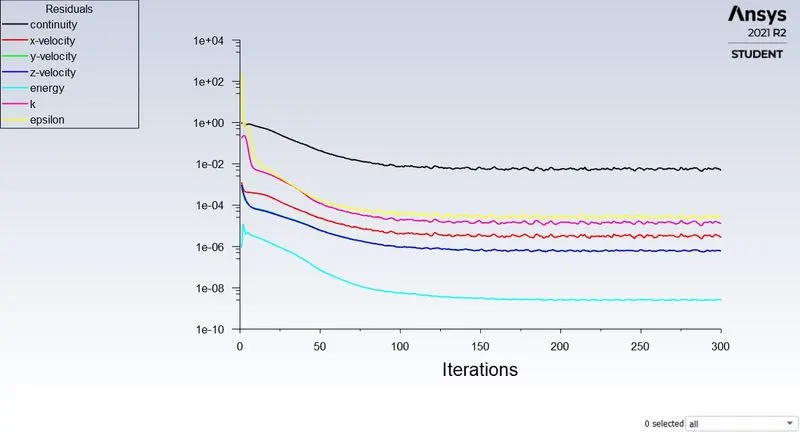
*We can see that solution has converged after about 200 iterations.
Temperature Contour -
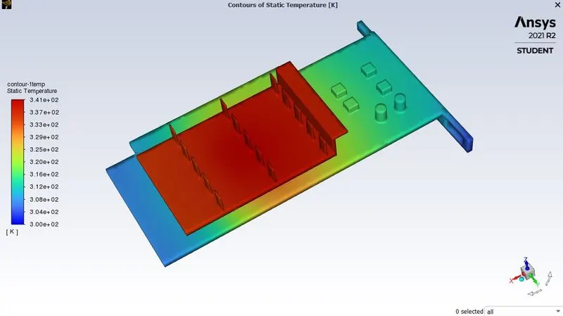
*Below is the plot for temperature contour.It can be observed that,high temperature regions around processor, which is mainly due to conduction
Heat Transfer Coefficient Contour -
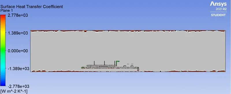
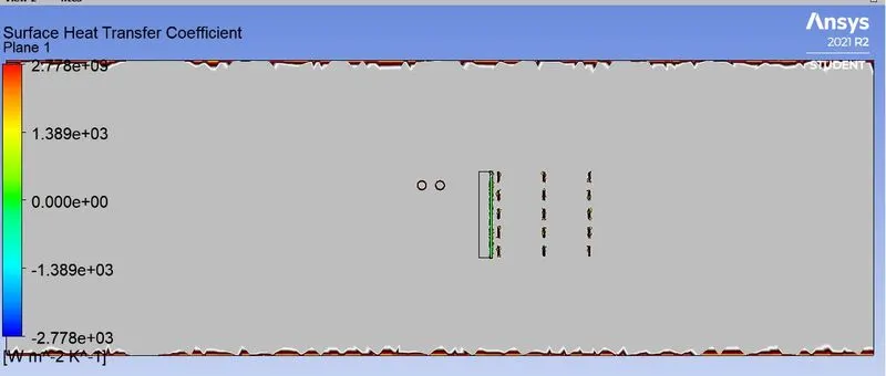
*Below is the plot for heat transfer coefficient contour on graphic card.We can see that maximum heat transfer due to convection is at the capacitors,which is mainly due to their shape,as heat transfer depends on area.It increases as the air velocity increases.
*Also as the fluid stream passes over the fins,intermixing takes palce and heat transfer increases.
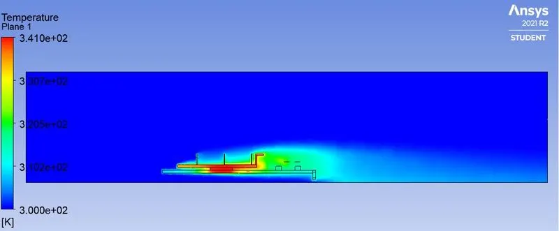
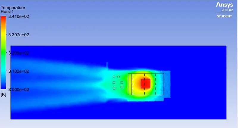
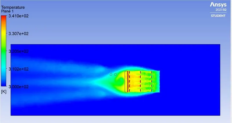
Plane Temperature Contour -
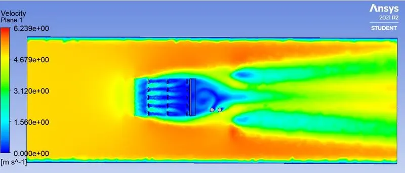
*Below is the plot for temperature contour on plane.It can be observed that,high temperature is at the end of the fins,this is mainly due to recirculation region.We can observe this clearly in velocity contour.
Plane velocity contour -
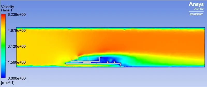
*In the below contour plot we can see that,velocity at the end of the fins is almost close to zero because of recirculation
region.The recirculation region can be visualized clearly in vector contour plot.
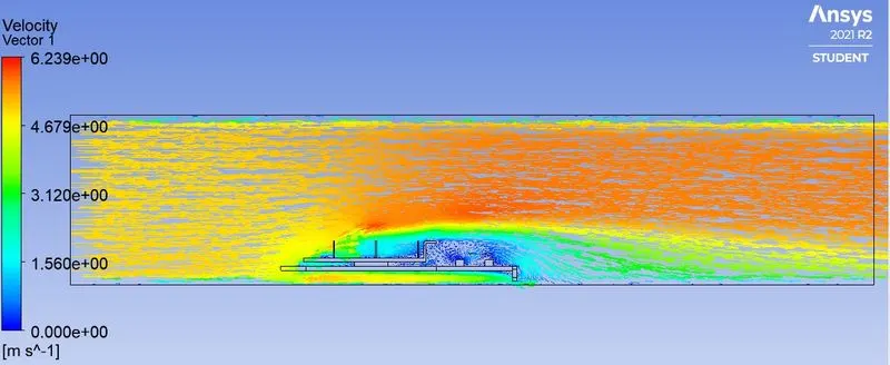
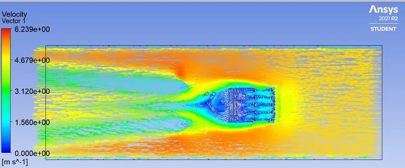
Plane velocity vector contour plot -
In the below plot velocity vectors are plotted on mid plane ,while temperature is plotted on midplane and graphic card.It
can be observed that,the places where temperature is high,is also the region of recirculation.
7] Verifying the HTC predictions from the simulations -
*The nusselt number is the ratio of convective to conductive heat transfer across a boundary.
Nu_L = convective heat transfer/conductive heat transfer = h/(k/L) = hL/k.
where, h - convective heat transfer coefficient of the flow
L - Characteriatics length
k - Thermal conductivity of the fluid
Also Nusselt number is releated to Reynolds Number(Re)
Nu_D = 0.023Re_D^4/5Pr_n
where, Re = uL/nu = rho*uL/mu
u = flow speed (m/s)
* If we observe heat transfer coefficient is directly proportional to the reynolds number(also to the velocity).So if you increase the velocity then there will be increase in the convective heat transfer coefficient.Thats what we have proved above.Also if we run another simulaton and increase reynolds number ,the heat transfer coefficient will increase.
| Velocity`m/s` | Maximum Processor Temperature(K) | Processor Surface Heat Transfer Coefficient(`W/(m^2K)` |
| 1 | 399.48838 | 405.21278 |
| 3 | 352.77635 | 591.07917 |
| 5 | 340.58609 | 674.80271 |
8] Potential Hotspots on the model -
*It can be observed from the plots of HTC and temperature that,the potential hotspots are at the cylidrical capactors,which is due to convection,and also due to their shape,as we heat transfer coefficient depends on area and also on velocity.As velocity
of air increases,coefficient of heat transfer also increases.
*Also hotspots are around processor,which is due to conduction.
*There is another hot spot in the recirculation region.So we should not put any component in that region to avoid failure.
9] Factors on which the accuracy of the prediction depends on -
*Need to choose the exact turbulence model.Since this study is wall boundes,it's best to use k-omegaSST model.
*Share topology should be set to share,to have conformal meshing for proper connectivity.
*Whenever inputing any values,give proper decimal values to avoide round off error.
*Set proper y+ value based on the turbulence model selected.
10] Conclusion -
*We have successfully performed, the CHT analysis on a graphic card.
*The heat transfer coefficient increases as the inlet velocity increases.
*Better cooling is observed at velocity of 5 m /s
*Verified our results using Nusselt number and Reynolds number relation.