Week 8 - Simulating Cyclone separator with Discrete Phase Modelling

1].Aim -

To perform analysis on cyclone separator and calculate the separation efficiency and pressure drop.

2].Objective -

*To write few words about four emperical models used to calculate the cyclone separator efficiency.
*To perform an analysis on a given cyclone separator model by varying the particle diameter from 1`mum`  to 5 `mum` and calculate the separation efficiency in each case and discuss the results.Use both flow and particle velocity as `3 m/sec`.
*To perform an analysis on a given cyclone separator model by varying the particle velocity from `1 m/s` to`3 m/s` and then
`5 m/s` and calculate the separation efficiency and pressure drop in each case and discuss the results.Use particle diameter
size as `5 mum` and keep flow and particle velocity same.

3].Introduction and Theory -

Cyclonic separation is a method of removing particulates from an air, gas or liquid stream, without the use of filters, through vortex separation. When removing particulate matter from liquid, a hydrocyclone is used; while from gas, a gas cyclone is used. Rotational effects and gravity are used to separate mixtures of solids and fluids. The method can also be used to separate fine droplets of liquid from a gaseous stream.

A cyclone separator has several colloquial names.These names include 'dust separator','dust collector','dust extractor',
'cyclone extractor' and 'cyclone separator'.Generally small units are referred as 'dust' separators or extractors,whilst large scale industrial separators are referred to as cyclone separators.

Gas cyclone separators are grouped into two main categories,reverse flow and axial flow.In this project we are using reverse
flow cyclone separator ,since they are the most commonly used.A high speed rotating (air)flow is established within a
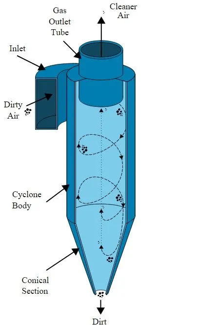
cylindrical or conical container called a cyclone. Air flows in a helical pattern, beginning at the top (wide end) of the cyclone and ending at the bottom (narrow) end before exiting the cyclone in a straight stream through the center of the cyclone and out the top. Larger (denser) particles in the rotating stream have too much inertia to follow the tight curve of the stream, and thus strike the outside wall, then fall to the bottom of the cyclone where they can be removed. In a conical system, as the rotating flow moves towards the narrow end of the cyclone, the rotational radius of the stream is reduced, thus separating smaller and smaller particles. The cyclone geometry, together with volumetric flow rate, defines the cut point of the cyclone. This is the size of particle that will be removed from the stream with a 50% efficiency. Particles larger than the cut point will be removed with a greater efficiency, and smaller particles with a lower efficiency as they separate with more difficulty or can be subject to re-entrainment when the air vortex reverses direction to move in direction of the outlet.

4].Formulae -

                                                                       
5].Pressure Drop -

DR = Ra Inlet - Ra Outlet - 1

Where,DR = Cyclone Pressure Drop
Ra = Absolute Pressure

Separation Efficiency -

`eta_s` = Number of Particles Trapped/Number of particles Tracked

6].Parameters for good cyclone Operation -

The following parameters are decisive for good cyclone operation -
*The Design
*The specific weight difference between two product phases
*The shape of the solids
*The speed of the feed
*The density of the medium
*The counter pressure at the overflow and apex.

7].Emperical Models Used for Cyclone Separator Efficiency -

                                                 

7.1].IOZIA AND LEITH MODEL

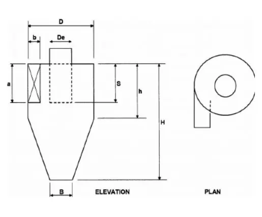
Iozia and Leith (1990) logistic model is a modified version of Barth (1956) model which is developed based on force balance. The model assumes that a particle carried by the vortex endures the influence of two forces: a centrifugal force, Z, and a flow resistance, W. Core length, zc, and core diameter,dc, are given as -

`z_c= (H-S)-[(H-S)/((D/B)-1)][(d_c/B)-1]` for `d_c > B`

`z_c = H-S` for `d_c < B`

`d_c= 0.47[(ab)/D^2]^-0.25*[D_e/D]^1.4`

The addition made by Iozia and Leith on the original Barth (1956) model are the core length zc and slope parameter β
expression which is derived based on the statistical analysis of experimental data of cyclone with D = 0.25 m. The collection
efficiency ηi of particle diameter dpi can be calculated from,

`ηi =1/(1+(d_(pc) / d_pi)^β`

where `d_(pc)` is the 50% cut size given by Barth (1956)

`d_(pc) = [9µQ/π*p_p z_c*v^2_t_max]^0.5`

7.2]. LI AND WANG MODEL

The Li and Wang (1989) model includes particle bounce or re-entrainment and turbulent diffusion at the cyclone wall. A
two-dimensional analytical expression of particle distribution in the cyclone is obtained. Li and Wang model was developed
based on the following assumptions:
• The radial particle velocity and the radial concentration profile are not constant, for uncollected particles within the cyclones.
• Boundary conditions with the consideration of turbulent diffusion coefficient and particle bounce re-entrainment on the
cyclone wall are:
`c = c_0` , at θ = 0

`D_r*∂_c/∂_r = (1- α)wc`, at`r = D/2`

• The tangential velocity is related to the radius of cyclone by:`uR^n` = constant.
The concentration distribution in a cyclone is given as:

`c(r, θ) =c_0(r_w− r_n) exp{−λ[1/(K (1+n))r^(1+n)]}/(int_(r_n)^(r_w)(exp{1/(K(1+n))*r^(1+n})dr`

Where,

`K =[(1 − n)(ρ_p− ρ_g)d^2Q]/(18 µb(r_w^(1−n)− r_n^(1−n))`

and

`λ =((1 − α)K w_w)/(D_r*r_w^n)`

The resultant expression of the collection efficiency for particle of any size is given as
`η_i= 1 − exp{−λθ_1}`
where
`θ_1= 2π (S + L)/a`

7.3]. Koch and Licht Model

Koch and Licht collection theory recognized the inher-ently turbulent nature of cyclones and the distribution of gas residence times within the cyclone. Koch and Licht described particle motion in the entry and collection regions with the additional following assumptions:
•The tangential velocity of a particle is equal to the tan-gential velocity of the gas flow, i.e. there is no slip in the
tangential direction between the particle and the gas.
•The tangential velocity is related to the radius of cyclone by: `u R^n`= constant.

A force balance and an equation on the particles collection yields the grade efficiency `η_i`

`η_i= 1 − exp{−2[Gτ_iQ/D^3 *(n + 1)]^(0.5/(n+1))}`
where
`G =8K_c/(K_a^2K_b^2)`
`n = 1 −{1 −(12D)^0.14/2.5}{(T + 460)/530}^0.3`
`tau_i=ρ_pd_pi^2/(18µ`

G is a factor related to the configuration of the cyclone, n is related to the vortex and τ is the relaxation term.

7.4]. Lapple Model

Lapple model was developed based on force balance with-out considering the flow resistance. Lapple assumed that a particle entering the cyclone is evenly distributed across the inlet opening. The particle that travels from inlet half width to the wall in the cyclone is collected with 50% efficiency. The semi empirical relationship developed by Lapple to calculate a 50% cut diameter, d_pc, is

`d_(pc)=[(9*µb)/(2π N_e v_i(ρ_p− ρ_g))]^(1/2`

where N_e is the number of revolutions
`N_e=1/a[h +(H − h)/2]`

The efficiency of collection of any size of particle is given by
`ηi=1/(1 + (d_(pc)/vecd_pi)^2`

8].Solution Procedure -

For simulating cyclone separator using DPM ,we will follow the below procedure :-

Geometry Creation --> Meshing --> Setup --> Solution & Post Processing

8.1].Geometry Creation -

                               

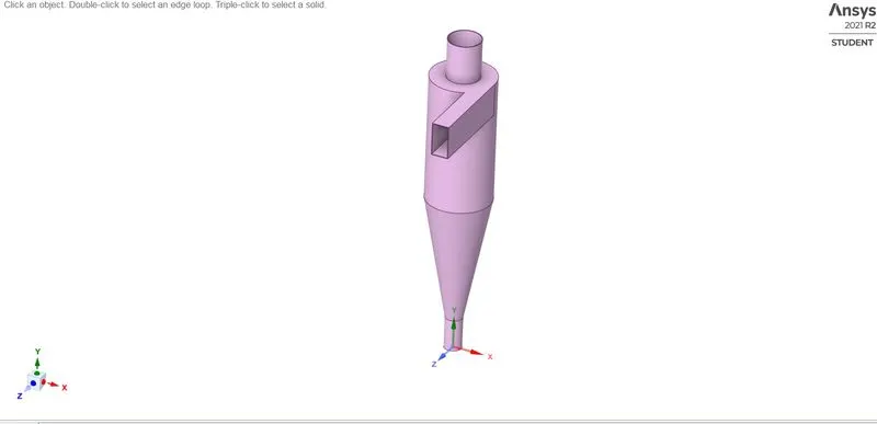
* Launch the Ansys workbench.First drag and drop the Fluid Flow(Fluent)model into project schematic and double click on geometry to launch the SpaceClaim.
* Import the geometry into the ansys spaceclaim.Below we can see the image of the 3D view of the cyclone separator model
used in this project.
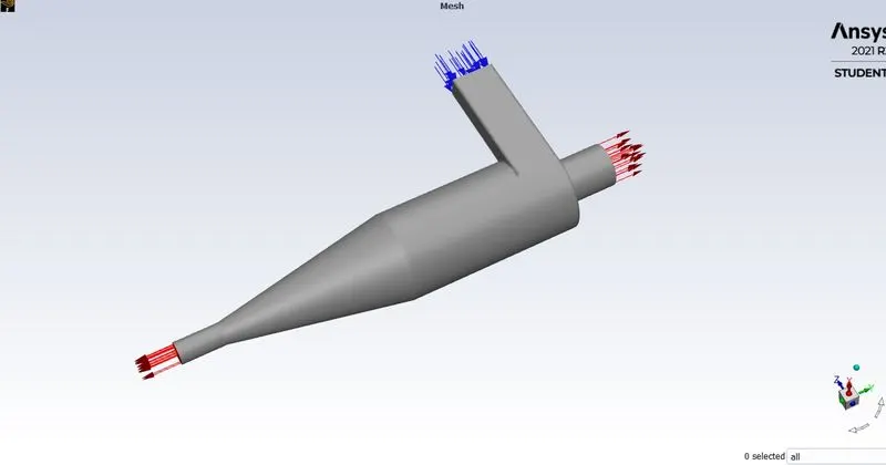
*It has one inlet on it's side,and two outlets one at bottom and other at the top.
*We need to extract fluid volume,for that follow the below procedure,
click Prepare => volume extract => select edge selection => select all inlet & outlet edges => ok.

                                       
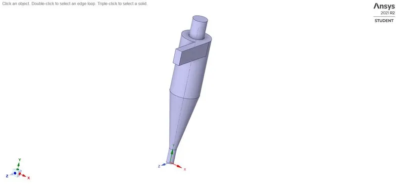
*Hide and supress the original cyclone separator geometry for physics.
*Close the spaceClaim.

8.2].Meshing -

*Now,go to meshing, by double clicking on mesh,and first do the name selection i.e give proper boundary names.Then generate the basic mesh using generate mesh command.We can see the flow of the mesh inside the extracted volume by using section plane.Also we can check the mesh quality by using mesh quality option.

select the prefered body => press N => name the selection.

*In meshing we can see the mesh is perfect.Always create the named selection first before generating the mesh.Select the edge you want to name,click N & name the selection.This way create named selection for inlet & both outlets.
*Then,next thing to do is to mesh.We click the mesh option in the side window and create our base line mesh.We then refine
mesh by giving element size as 5 mm and enable programme controlled inflation.
*Below is the geometry with final mesh.

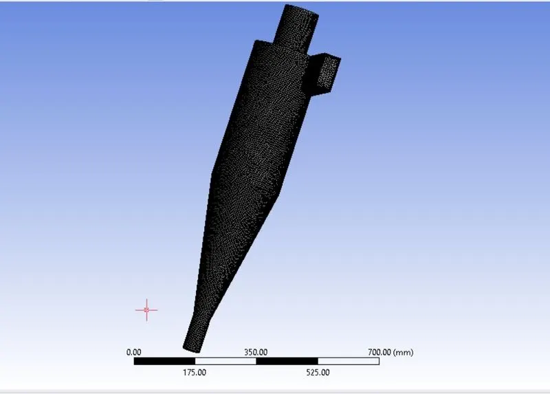
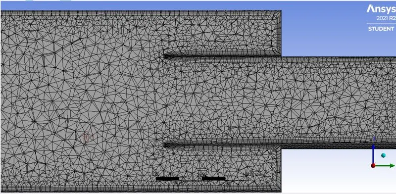
* Now lets check our mesh quality.Our minimum mesh quality is good enough.
* This concludes our meshing procedure.
* Now close the mesh & update.

8.3].Setup -

* Double click setup in project schematic.This will open ansys fluent.

*In the below image we can see inlet shaded as blue and outlet shaded as red.

*Click on check mesh and make sure there are no errors.

                                          

8.3.1].Setting up Physics

*Our solution method will be SIMPLE.
*We will use second order upwind for turbulent kinetic energy and turbulent dissipation rate.

8.3.2].General -

*Solver type - pressure based
*time - Steady state
*velocity formulation - absolute
* We need to enable gravity.Since our geometry is in XY-plane,give negative value for acceleration due to gravity.
General => Gravity =>Gravitational acceleration => Y(m/s) = -9.81 m/s.

8.3.3].Models -

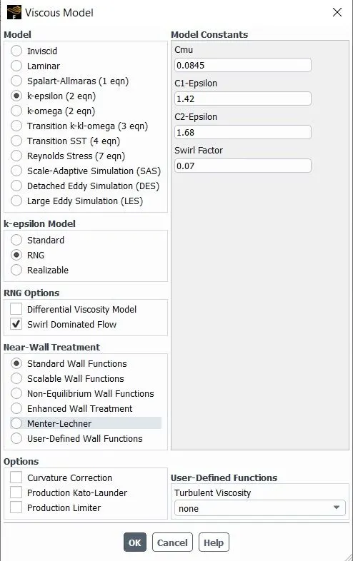
*viscous model - k-epsilon RNG model
*RNG options - swirl dominated flow

RNG is the slight modification of standard model.It enhances the accuracy of swirlng flows.

                                                 

8.3.4].Material -

*Fluid - Air

8.3.5].Discrete Phase Modelling(DPM) Setup -

There are two ways of carrying out DPM -
1).Uncoupled Flow - Discrete phase will not have any interaction with continuous phase
2).Coupled Flow - The discrete phase will influence the flow of the continuous phase.
Since size of the particles injected into the cyclone separator is very small,usage of both type of flow shouldn't matter much.
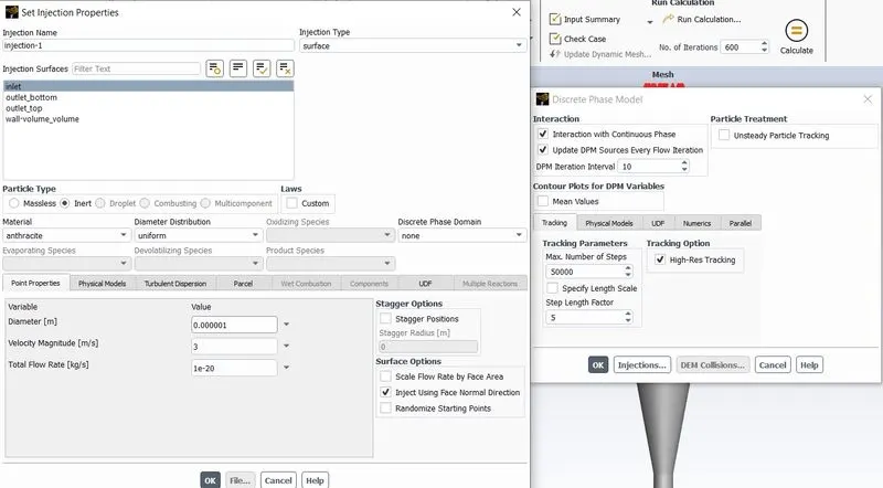
In Models =>Click on Discrete Phase =>
1) select interaction with continuous phase and also update DPM sources every flow iterations.
2) set DPM iteration interval = 10
3)Tracking => Tracking parameters => keep all the default values.

8.3.6].*Now we have to specify the injections of the discrete particles on to the continous phase.To do this follow below steps -

Models => Discrete Phase => click on Injection => create =>
1)particle type => inert
2)Material => Anthracite
3)Injection Type => Surface
4)Release from surfaces => Inlet
5)Point Properties => A] x-velocity = 3m/s(This will act normally to the above selected surface)
                                B] Diameter = 1e-6 m
6)Close discrete phase modelling.

       

8.3.7].Boundary conditions - We can see all the named selections which,we generated above being used as boundary conditions.

         

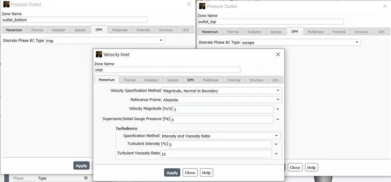
* Inlet -
Type - velocity inlet
velocity magnitude - 3m/sec
DPM - reflect

* Outlet Top -
Type - pressure outlet
gauge pressure - 0 Pa
DPM - escape

* Outlet Bottom -
Type - pressure outlet
gauge pressure - 0 Pa
DPM - trap
*Now we will initialize from the inlet with standard initialization.

8.3.8].Solving -

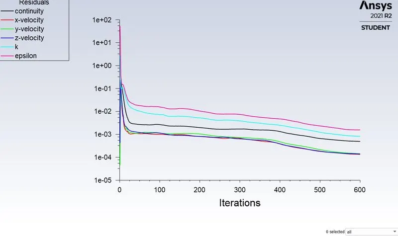
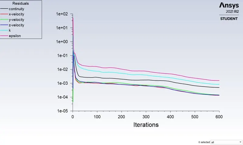
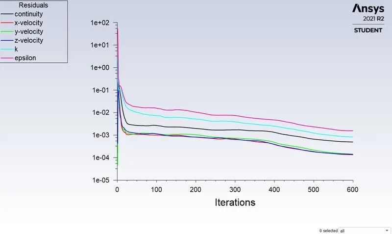
*Run the simulation for 600 iterations
*After completing the calculation,we need to export the particle tracking data for that,
File => export => Particle History Data => Select injection =0 =>click on browse give particle file name => ok => write.
*In the console we can see total number of particles tracked.

8.4].Solution & Post Processing -

*Launch the CFD post by double clicking on Results in project schematic.
*First import particle tracking data-
File => import => Import fluent particle track file => browse the file => ok
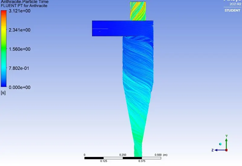
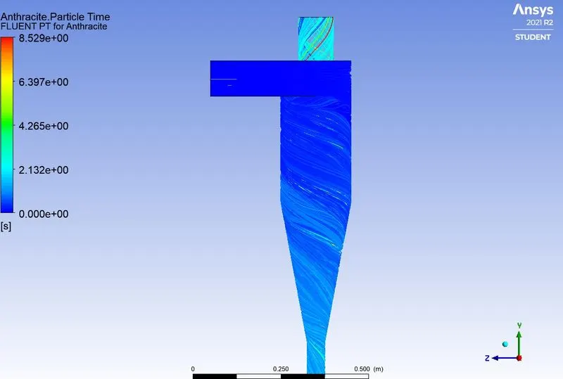
*We can see fluent PT for anthracite in the user locations and plots.

Residual Plot -

                                     
Anthracite Particle Time Contour -

                                   
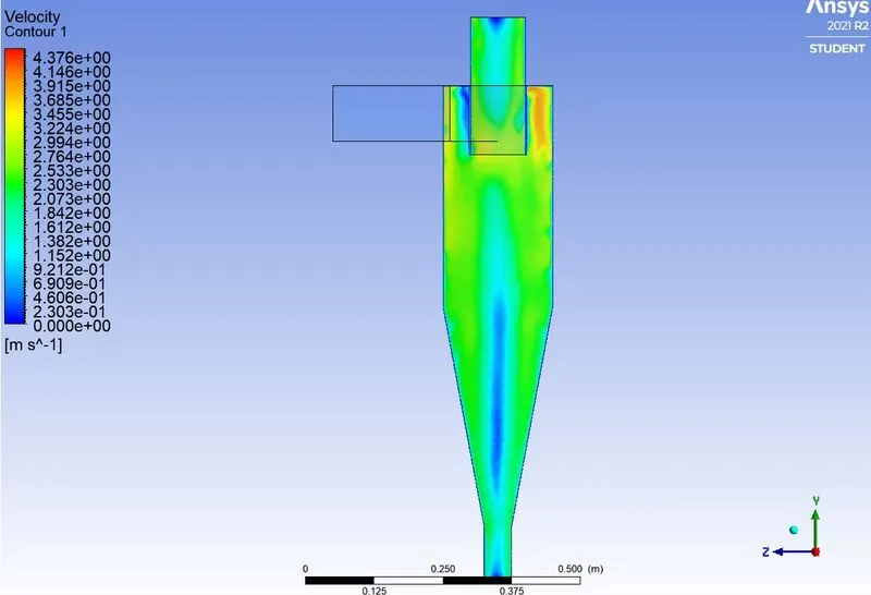
Velocity contour -

                                    
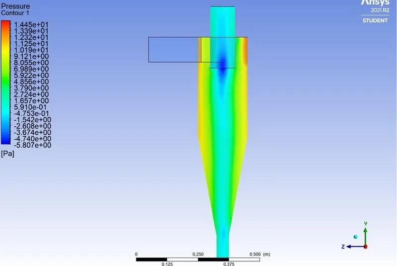
Pressure Contour -

                                   
Animation -

https://www.youtube.com/watch?v=puZ708ALApI

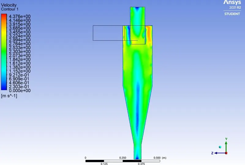
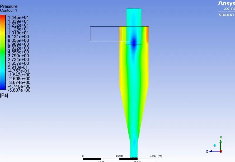
Now lets simulate for other two cases with different with different particle diameter and with same fluid and particle velocity.

8.4.1].Particle Diameter of 3 um -

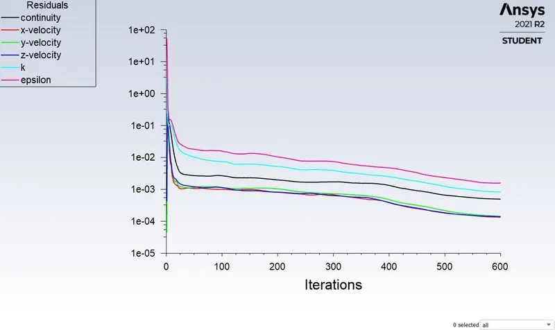
Residual Plot -

                                    
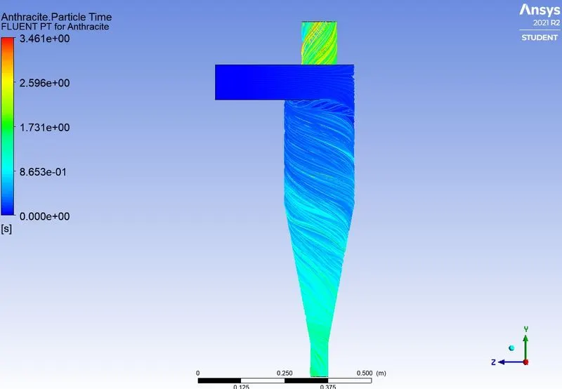
Anthracite Particle Time Contour -

                                    
Velocity contour -

                                    
Pressure Contour -

                                   
Animation -

https://www.youtube.com/watch?v=WjNRxJl7IIc 

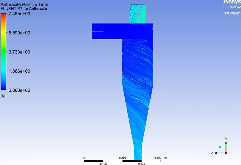
8.4.2].Particle Diameter of 5 um -

Residual Plot -

                               
Anthracite Particle Time Contour -

                                
Velocity contour -

                                
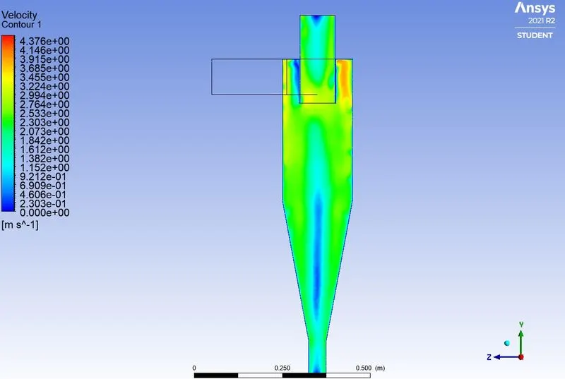
Pressure Contour -

                                 
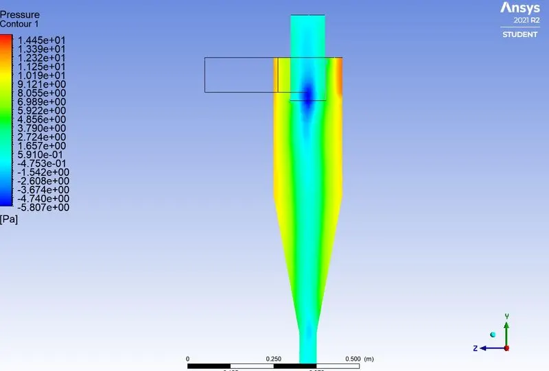
Animation -

https://www.youtube.com/watch?v=pJ_vpbVztuw

Compairing Above Cases -

Particle Diameter	Tracked	Escaped	Trapped	Separation Efficiency
5 `mum`	470	84	386	0.8212
3 `mum`	470	155	315	0.6702
1 `mum`	470	205	265	0.5638

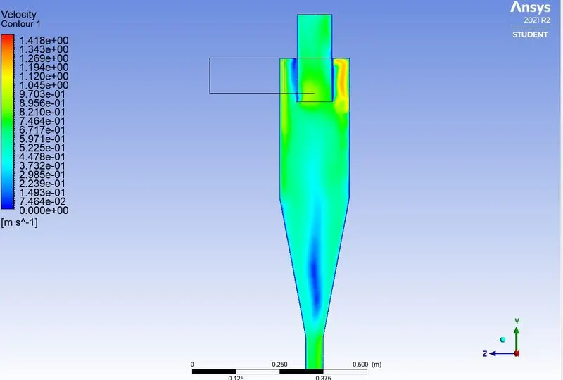
*From the above table we can observe that, as the particle diameter is increasing so does the number of particles trapped at
the bottom outlet,thus increasing the separation efficiency of the cyclone separator.

9].Analysis of cyclone separator at same particle diameter but with varying particle velocities -

*Now we will perform an analysis on a given cyclone separator model by varying the particle velocity from `1 m/s to 5 m/s`
and will calculate separation efficiency and pressure drop in each case .Then will compare them.

9.1].Particle Velocity of 1 m/s -

Residual Plot -

                                   
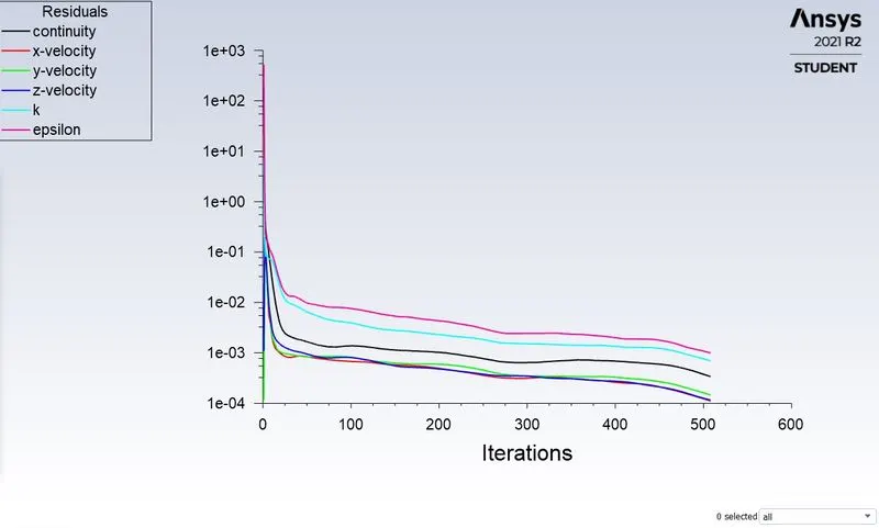
Anthracite Particle Time Contour -

                                    
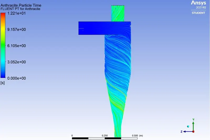
Velocity contour -

                                 
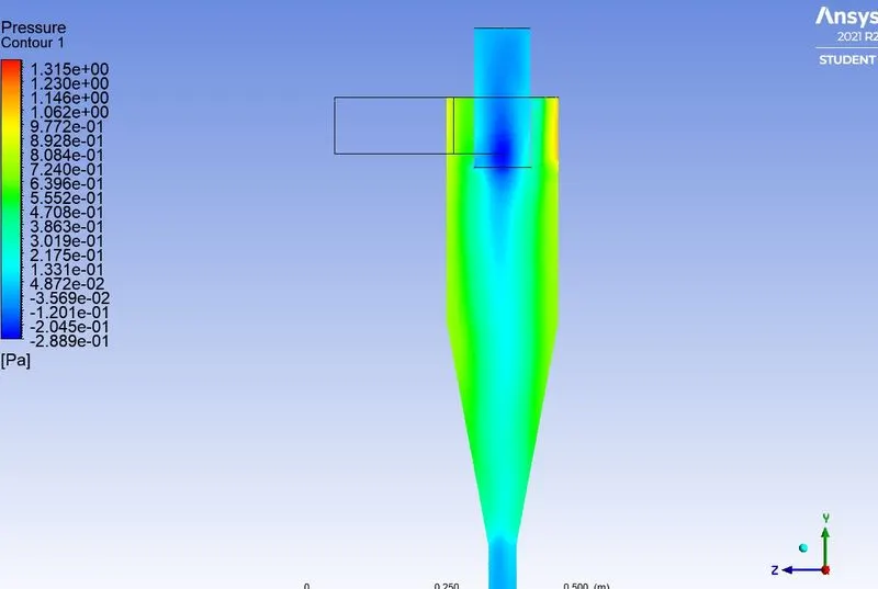
Pressure Contour -

                                 
Animation -

https://www.youtube.com/watch?v=EmdrsskEHOo 

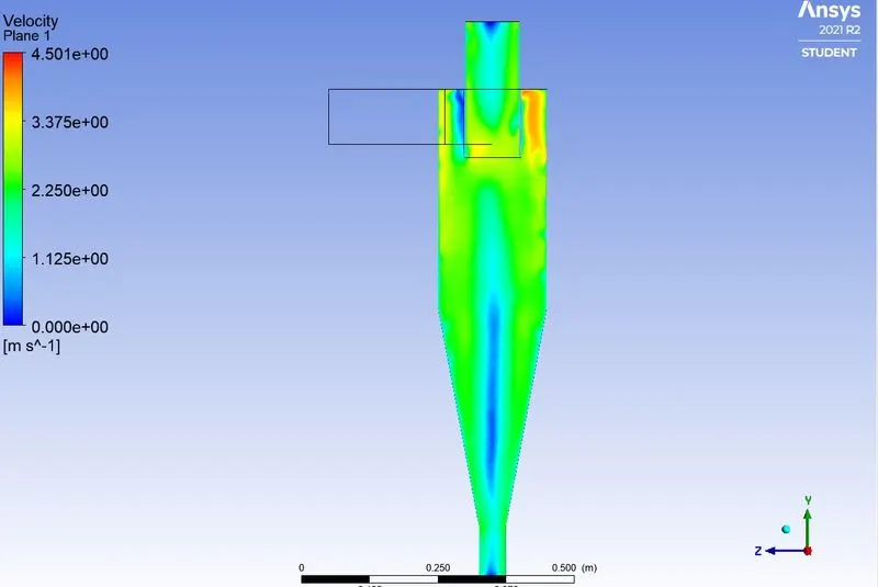
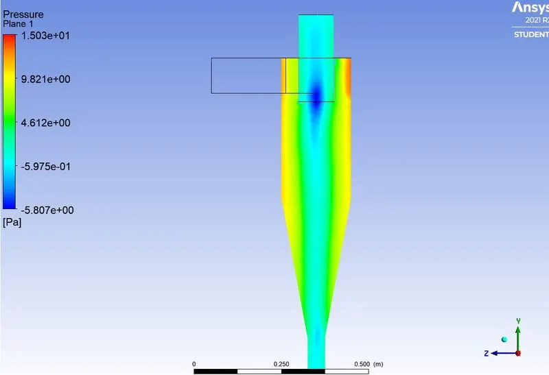
9.2].Particle Velocity of 3 m/s -

Residual Plot -

                             
Anthracite Particle Time Contour -

                              
Velocity contour -

                               
Pressure Contour -

                               
Animation -

 https://www.youtube.com/watch?v=hjqpibZYljk

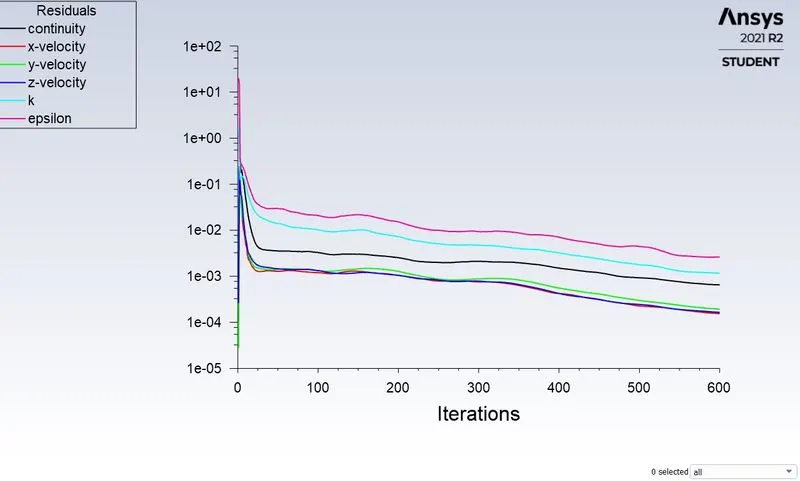
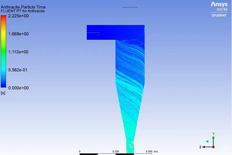
9.3].Particle Velocity of 5 m/s -

Residual Plot -

                           
Anthracite Particle Time Contour -

                             
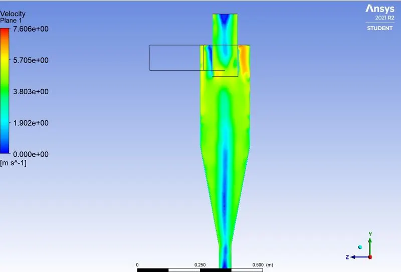
Velocity contour -

                             
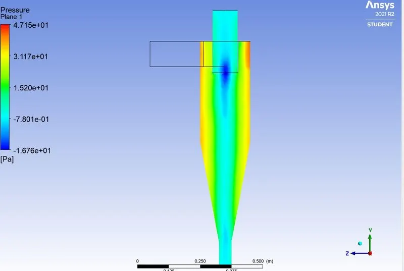
Pressure Contour -

                             
Animation -

https://www.youtube.com/watch?v=LKrJ3mYEA1o 

Compairing Above Cases -

Particle Velocity(`m/s`)	Tracked	Escaped	Trapped	Separation Efficiency	Pressure Drop(Pa)
5 `m/s`	470	0	470	1	55.7475
3`m/s`	470	84	386	0.8212	18.4786
1`m/s`	470	211	259	0.5510	1.6057

*From the above table we can observe that, as the particle velocity is increasing so does the number of particles trapped at the bottom outlet,thus increasing the separation efficiency of the cyclone separator.Also pressure drop increases with increase in velocity

10].Conclusion -

*Particle size and velocity is the dominating factor in the separation efficiency.Large particles can be separated easily compared to small particles.
*As the velocity increases,separation efficiency and pressure drop increases.
*Centrifugal force dominates over resistance or drag force as the velocity increases.