Week 8 - Simulation of a backward facing step in OpenFOAM
Aim -
To simulate 2D transient CFD simulation of an incompressible, laminar viscous flow over the backward facing step in OpenFoam, by first creating a non grading mesh and then graded mesh.
Explaination -
Consider a 2D laminar,incompressible flow over the backward facing step.The geometry of the backward facing step is shown in the following figure.Consider no-slip boundary condition on every wall.We will perform a transient 2D simulation using openfoam by first creating a non grading mesh and then graded mesh,to observe the effect of grading factor on final results.
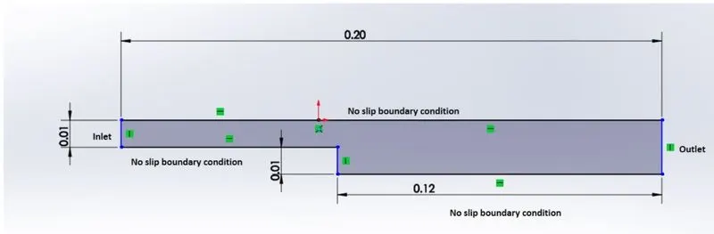
In the results,we need to create the velocity contour and plots of velocity near the step,for each grading factor,to observe their effects.Assume constant velocity inlet and constant zero gauge pressure outlet as the initial boundary conditions.As the flow velocity depends on Reynolds number,and our flow is laminar,hence consider Reynolds number as 2100.We will run the simulation for 40 sec.This simulation will be carried out with the aid of tutorial named cavity under the icoFoam solver.
Simulation Procedure -
Choosing the Solver :
To simulate the the given problem,we first need to choose the appropriate openfoam tutorial,that suits our problem statement.I chose icoFoam solver,under incompressible tutorials.icoFoam is a PISO loop based solver.It is a transient laminar incompressible solver.The flow will therefore be solved transiently until the steady state is obtained.
Geometry & Mesh :
The blockMesh utility is used to-
* create geometry by building blocks from the co-ordinates of their vertices.
* generate a structured mesh by defining the number of nodes for each main direction.
* create the patches for each of the boundary conditions.
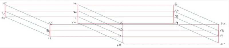
The geometry is divided into ten blocks.For this purpose 22 vertices are defined in the blockMesh dictionary.The blocks(nodes 0 to 5) and blocks(11 to 16) are used to create the upstream portion of the step.And block(10 9 8 1 21 20 19 14) is used to create the lower part of the channel,downstream of the step.The dictionary has following lines to create the mesh.After defining the different nodes necessary for the mesh,the patches of the domain are also created in the blockMesh file.Because the problem is modeled with 2D flow assumption,out of plane patches are defined with an empty type.
/*--------------------------------*- C++ -*----------------------------------*\
  =========                 |
  \\      /  F ield         | OpenFOAM: The Open Source CFD Toolbox
   \\    /   O peration     | Website:  https://openfoam.org
    \\  /    A nd           | Version:  9
     \\/     M anipulation  |
\*---------------------------------------------------------------------------*/
FoamFile
{
    format      ascii;
    class       dictionary;
    object      blockMeshDict;
}
// * * * * * * * * * * * * * * * * * * * * * * * * * * * * * * * * * * * * * //

// Note: this file is a Copy of $FOAM_TUTORIALS/resources/blockMesh/pitzDaily

convertToMeters 1;

vertices
(
    ( 0 0 0)
    (0.08 0 0)
    (0.08 0.005 0)
    (0 0.005 0)
    (0.08 0.01 0)
    (0 0.01 0)
    (0.2 0.01 0)
    (0.2 0.005 0)
    (0.2 0 0)
    (0.2 -0.01 0)
    (0.08 -0.01 0)

    (0 0 0.03)
    (0.08 0 0.03)
    (0.08 0.005 0.03)
    (0 0.005 0.03)
    (0.08 0.01 0.03)
    (0 0.01 0.03)
    (0.2 0.01 0.03)
    (0.2 0.005 0.03)
    (0.2 0 0.03)
    (0.2 -0.01 0.03)
    (0.08 -0.01 0.03)
);


blocks
(
    hex (0 1 2 3 11 12 13 14) (200 10 1) simpleGrading (1 1 1)

  hex (3 2 4 5 14 13 15 16) (200 10 1) simpleGrading (1 1 1)

  hex (2 7 6 4 13 18 17 15) (200 10 1) simpleGrading (1 1 1)

  hex (1 8 7 2 12 19 18 13) (200 10 1) simpleGrading (1 1 1)

  hex (10 9 8 1 21 20 19 12) (200 10 1) simpleGrading (1 1 1)
);

edges
(
);

boundary
(
    inlet
    {
        type patch;
        faces
        (
            (0 11 14 3)
            (3 14 16 5)
        );
    }
    outlet
    {
        type patch;
        faces
        (
            (9 8 19 20)
            (8 7 18 19)
            (7 6 17 18)
        );
    }
    TopandBottomfaces
    {
        type wall;
        faces
        (
            (5 4 15 16)
            (4 6 17 15)
            (0 11 12 1)
            (10 21 20 9)
            (1 12 21 10)
        );
    }

    frontAndBack
    {
        type empty;
        faces
        (
            (0 1 2 3)
            (3 2 4 5)
            (4 2 7 6)
            (2 1 8 7)
            (1 10 9 8)
            (14 13 12 11)
            (14 16 15 13)
            (13 15 17 18)
            (12 13 18 19)
            (21 12 19 20)
        );
    }
);
mergePatchPairs
(
);

// ************************************************************************* // 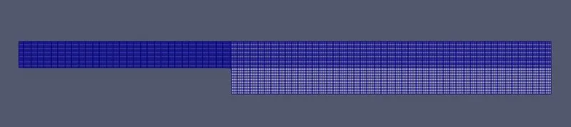
Fig - Mesh with Grading Factor 1
Boundary Condition :
The boundary conditions used are standard :
*Inlet - constant velocity and zero pressure gadient
*Outlet - zero velocity gradient and static pressure set to 0 Pa.
*Walls - zero pressure gradient
The laminar flow velocity is calculated using Reynolds number formula as follows,
`R_e = UL/nu`
`U=R_e*nu/L`
Where,
`R_e` = Reynolds number
U = Initial velocity
L = Characteristics length of the domain
`nu` = Kinematic viscosity
`U=2300*10^-6/0.2`
U = 0.0105 m/sec
Initial Velocity Condition :
/*--------------------------------*- C++ -*----------------------------------*\
  =========                 |
  \\      /  F ield         | OpenFOAM: The Open Source CFD Toolbox
   \\    /   O peration     | Website:  https://openfoam.org
    \\  /    A nd           | Version:  9
     \\/     M anipulation  |
\*---------------------------------------------------------------------------*/
FoamFile
{
    format      ascii;
    class       volVectorField;
    object      U;
}
// * * * * * * * * * * * * * * * * * * * * * * * * * * * * * * * * * * * * * //

dimensions      [0 1 -1 0 0 0 0];

internalField   uniform (0 0 0);

boundaryField
{
    inlet
    {
        type            fixedValue;
        value           uniform (0.0105 0 0);
    }

outlet
{
type			zeroGradient;
}
    TopandBottomfaces
    {
        type            noSlip;
    }

    frontAndBack
    {
        type            empty;
    }
}

// ************************************************************************* //
Initial Pressure Condition :
/*--------------------------------*- C++ -*----------------------------------*\
  =========                 |
  \\      /  F ield         | OpenFOAM: The Open Source CFD Toolbox
   \\    /   O peration     | Website:  https://openfoam.org
    \\  /    A nd           | Version:  9
     \\/     M anipulation  |
\*---------------------------------------------------------------------------*/
FoamFile
{
    format      ascii;
    class       volScalarField;
    object      p;
}
// * * * * * * * * * * * * * * * * * * * * * * * * * * * * * * * * * * * * * //

dimensions      [0 2 -2 0 0 0 0];

internalField   uniform 0;

boundaryField
{
    inlet
    {
        type            zeroGradient;
    }

    outlet
     {
        type			fixedValue;
       value			uniform 0;
       }

    TopandBottomfaces
    {
        type            zeroGradient;
    }

    frontAndBack
    {
        type            empty;
    }
}

// ************************************************************************* //
Physical Properties :
The physical parameters for the specific flow problem are described in the file called TransportProperties file.This filr is located in the constant directory.In our case, we assume that our fluid is water and kinematic viscosity of water is given as 1e-6 m^2/sec.This file will be same for all analysis with different grading factor.
/*--------------------------------*- C++ -*----------------------------------*\
  =========                 |
  \\      /  F ield         | OpenFOAM: The Open Source CFD Toolbox
   \\    /   O peration     | Website:  https://openfoam.org
    \\  /    A nd           | Version:  9
     \\/     M anipulation  |
\*---------------------------------------------------------------------------*/
FoamFile
{
    format      ascii;
    class       dictionary;
    location    "constant";
    object      transportProperties;
}
// * * * * * * * * * * * * * * * * * * * * * * * * * * * * * * * * * * * * * //

nu              [0 2 -1 0 0 0 0] 1e-6;


// ************************************************************************* //
Timestep Value :
We want our numerical scheme to be accurate and stable.A scheme is stable,when truncation error does not increase in amplitude after each time step.So,there exist a stability criteria,for our problem,we use CFL stability criteria to set the stability condition.The input data relating to the control of time is read from controlDict.To have a stable solution CFL number should be less than 1.
The following calculations are done to get proper time step,
1) First smallest cell size dx is calculated
`dx=d/n=0.005/10=0.0005`
2) Then time step size(dt) is calculated
`dt=C_o*dx/U`
`dt = 0.047`
where,
`C_o`= Courant Number
So the time step must be less than 0.047 to have a stable solution.We can further verified our calculation ,by using CFL formula used in OpenFoam,
`C_o=Deltat*tau`
`C_o=0.89`
where,
`Deltat`=time step size
`tau` = characteristics time scale for the volumetric flux
Furthermore ,we can also calculate the time required for the flow to cover a distance equal to the characteristics length as follows,
`time(t)= L/U`
t= 19.05 sec
So we will run our simulation for 20 sec or more.
/*--------------------------------*- C++ -*----------------------------------*\
  =========                 |
  \\      /  F ield         | OpenFOAM: The Open Source CFD Toolbox
   \\    /   O peration     | Website:  https://openfoam.org
    \\  /    A nd           | Version:  9
     \\/     M anipulation  |
\*---------------------------------------------------------------------------*/
FoamFile
{
    format      ascii;
    class       dictionary;
    location    "system";
    object      controlDict;
}
// * * * * * * * * * * * * * * * * * * * * * * * * * * * * * * * * * * * * * //

application     icoFoam;

startFrom       startTime;

startTime       0;

stopAt          endTime;

endTime         40;

deltaT         0.04;

writeControl    timeStep;

writeInterval   50;

purgeWrite      0;

writeFormat     ascii;

writePrecision  6;

writeCompression off;

timeFormat      general;

timePrecision   6;

runTimeModifiable true;


// ************************************************************************* //
Post Processing :
The primary post processing tool provided with OpenFoam is ParaView.The results that are written in the time directories can be viewed using ParaView.To launch ParaView a command called paraFoam is used from within the case directory. paraFoam is a script file, which launches ParaView.We need to obtain plot of velocity profile near the step region.
Mesh Stretching or Mesh Refinement
Now to capture the boundary layer effect it is necessary to use finer mesh near the walls.The process of changing mesh,according to the physical need of the problem,in order to produce more accurate results, is called as mesh refinement.We are going to make our mesh finer near the wall by using non-zero grading factors in the blockMeshDict file known as simple grading.For our problem we are going to take grading factor of 0.2.
Mesh Grading -
blocks
(
    hex (0 1 2 3 11 12 13 14) (200 10 1) simpleGrading (0.2 1.2 1)

  hex (3 2 4 5 14 13 15 16) (200 10 1) simpleGrading (0.2 0.2 1)

  hex (2 7 6 4 13 18 17 15) (200 10 1) simpleGrading (1.2 0.2 1)

  hex (1 8 7 2 12 19 18 13) (200 10 1) simpleGrading (1.2 1.2 1)

  hex (10 9 8 1 21 20 19 12) (200 10 1) simpleGrading (1.2 1 1)
); 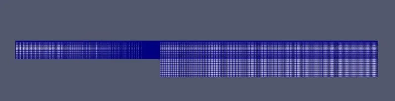
Fig. - Mesh After 0.2 Grading Factor
Why grading/growth factor is essential for meshing ?
In our problem ,we are dealing with laminar flow,so it becomes utmost importance to capture the boundary layer effect to get more accurate results.Boundary layer is the layer of fluid in the immediate vicinity of the bounding surface,where the effect of viscocityis significant. We can make our mesh finer near the walls,either by inreasing the number of cells in each block or by introducing the non zero grading factor.The latter way is preferred because,it is mre efficient.It gives more accurate results with a fewer number of cells than the former method,thereby decreasing the computational time.
Results And Conclusion -
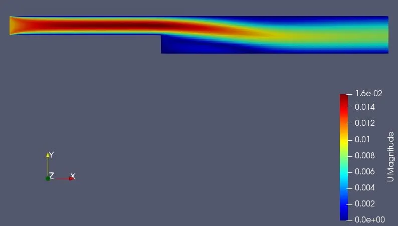
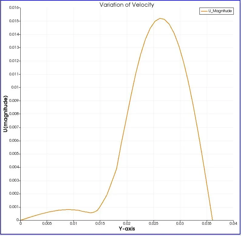
Result of Non Graded Mesh
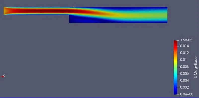
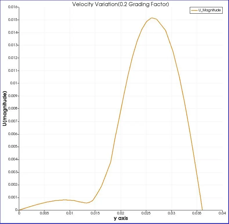
Result of Graded mesh with 0.2 as grading factor
Conclusion :
From the plots at 0.085 m ,we can see that,velocity near the walls is zero,whereas at the center it is maximum.This is due to no slip boundary condition at the walls.This make sense,beacause as the fluid is viscous,thus there is resistance between layers.Therefore velocity should be maximum near the center.
Also,we can observe that as simple grading is increasing,the velocity magnitude curve at a distance is becoming more smoother.