Week 10 - Simulating Combustion of Natural Gas.
1] Aim :-
To perform a non-premixed combustion simulation of natural gas on a combuster model.
2] Objective :-
1] Perform a comustion simulation on the combuster model and plot the variation of the mass fraction of the different
species in the simulation using line probes at different locations of the combuster.Plot for CO2,H2O,CH4,N2,O2,NOx emissions and soot formation.
2] In this part,we add the water content in the fuel from 5% to 30 % by mole and observe the effect of it on the results.We
provide line plots and contours to prove our claim.We use the parametric study approach for this part.
3] Introduction and Theory :-
Combustion or burning is a high temperature exothermic redox chemical reaction between a fuel(the reductant) and an oxidant,usually,atmospheric oxygen.Complete combustion is stoichiometric concerning the fuel,where there is no remaininfuel,and ideally no residual oxidant.Thermodynamically,the chemical equilibrium of combustion in air is overwhelmingly on the side of the products.
However,complete combustion is almost impossible to achieve,since the chemical equilibrium is not necessarily reached,or may contain unburnt products such as carbon monoxide,hydrogen and even carbon(soot or ash).Any combustion at high temperatures in atmospheric air,which is 78% nitrogen,will also create samll amounts of several nitrogen oxides,commonly referred to as NOx.Thus the produced smoake is usually toxic,and contains unburned or partially oxidized products.
In this study,we will observe the burning of methane in the air inside a cylindrical combustor using the eddy dissipation model in Ansys.Here the source them was modelled using the eddy dssipation model where the begining of the ignition is calculated using the turbulent time scale.This means that the ignition will start when and where there is turbulence.This is a crude approximation bus helps us to visualise the steady state temperature distribution in the combustion chamber at the faster rate.This type of mixing based model is called a turbulence chemistry interaction(TCI)model.
4] Solution Procedure -
For simulating combustion of natural gas ,we will follow the below procedure :-
Geometry Creation --> Meshing --> Setup --> Solution & Post Processing
4.1] Geometry Creation -
* Launch the Ansys workbench.First drag and drop the Fluid Flow(Fluent)model into project schematic and double click on geometry to launch the SpaceClaim.
* Import the geometry in to the ansys spaceclaim.
*Below is the 3D geometry of the combuster model.We won't be simulating the 3D model because of the limitations of the ansys academic version.So we need to extrat the 2D geometry from the given 3D model.
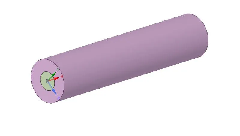
*Now we have to extract 2D geometry in the middle plane,for that we need to split the geometry in half.
*First create plane, in Design tab => select plane => click on origin(this will create three planes).
*Now to split the body,in Design => click on Split Body => first select targrt object i.e. extracted volume => select XY-plane to cut the body in half => click on the region to be removed i.e. front region.
*We can see the internal sectional view.When we select the top part of the remaining geometry,we can see yellow top face part, which is what we want.To extract this area,select face & copy it.Now open new design moduler and paste it there and save it.
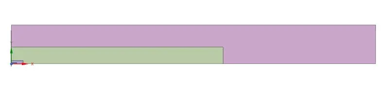
*In project schematic reset geometry and import the saved 2D geometry.
*Now we need to combine all the parts in the design.To do that drag a box around design then select combine from the above toolbox.Below is the final 2D geometry.

*Close the spaceclaim.
4.2] Meshing -
*Now,go to meshing, by double clicking on mesh,and first do the name selection i.e give proper boundary names.Then generate the basic mesh using generate mesh command.
*First give the name selection,select edge selection tool => click on top edge of the geometry => press N => name it as wall. In similar way give the named selection for air inlet,fuel inlet,axis,outlet.
*To mesh the geometry,click on mesh => element size = 1 mm => set proximity to on =>generate mesh.

* Now lets check our mesh quality.Our minimum mesh quality is good enough.
* This concludes our meshing procedure.
* Now close the mesh & update.
4.3] Setup -
* Double click setup in project schematic.This will open ansys fluent.
*Click on check mesh and make sure there are no errors.
4.3.1] Setting up Physics
Our solution method will be Coupled.
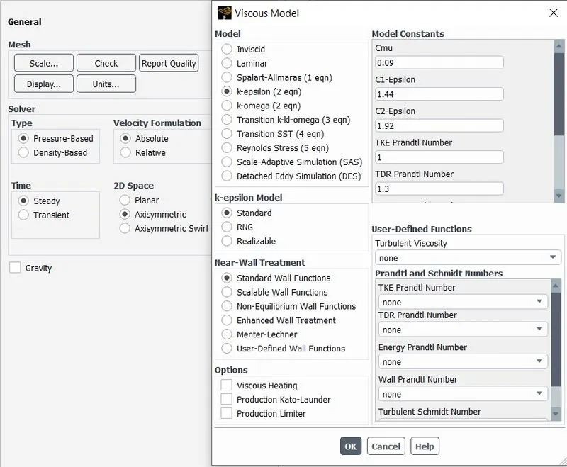
4.3.2] General -
*Solver type - pressure based
*time - Steady state
*velocity formulation - absolute
*2D space - Axisymmetric
*Energy - Enable
4.3.3] Models -
*viscous model - k-epsilon standard with standard wall function
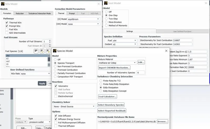
*Species model -
model - species transport
Reactions - Volumetric
*Options -select inlet diffusion and diffusion energy source.
*Mixture Properties -mixture material - methane-air -2 Step.
*Turbulence chemistery interarion - eddy dissipation.
*soot -one step soot model
*NOx - thermal NOx
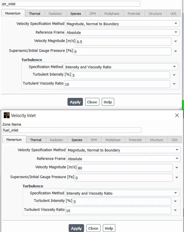
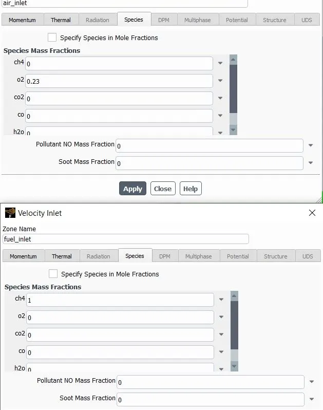
4.3.4] Boundary conditions - We can see all the named selections which,we generated above being used as boundary conditions.
* air inlet -
Type - velocity inlet
Velocity magnitude - 0.5 m/s
Thermal - 300 K
Species - In species mass fraction ,give O2 = 0.23 & set remaining species to zero.
*Fuel inlet -
Type - velocity inlet
Velocity magnitude - 80 m/s
Thermal - 300 K
Species - In species mass fraction ,give CH4 = 1 & set remaining species to zero.
* Outlet -
Type - pressure outlet
gauge pressure - 0 Pa
* wall - Type wall
* axis -Type axis
*Now we want moniter the flow quantities as the solution is being solved.We want to moniter temperature,soot and NOx at
the outlet.To do this follow the below steps,
In solutions tab => click definitions => new => surface report => area weighted average => select temperature as field variable and under it as static temperature => in surfaces select outlet => check report file & report plot => ok
*Now initialize the domain.We will use hybrid initialization,this provides very good initial conditions.
*For temperature contour go to postProcessing => contours => new => contour of => temperature => under it static temperature => select outlet => save/display.
Simillarly create contour for mass fraction of NOx,soot,CH4,CO2,H2O,N2,O2.
*To create animation,go to activities => solution animation => select temperature contour => preview => set desired view => give name as temperature animation.
4.4] Solving -
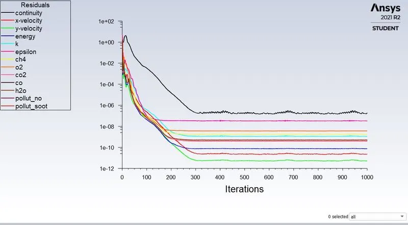
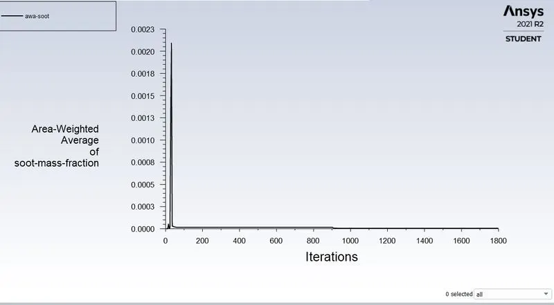
* We will run the simulation for 1000 iterations.We can see from the residual plot that our solution has converged and reached the steady state.
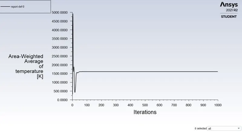
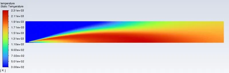
Area Weighted Average of Temperature At The Outlet -
The value of temperature at the outlet is 1611.1809 K.
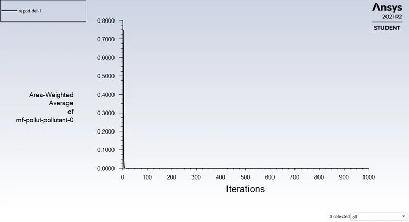
Area Weighted Average of Mass Fraction Of NOx At The Outlet -
The value of mass fraction of NOx at the outlet is 0.0001020.
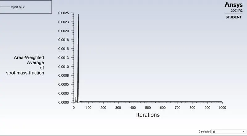
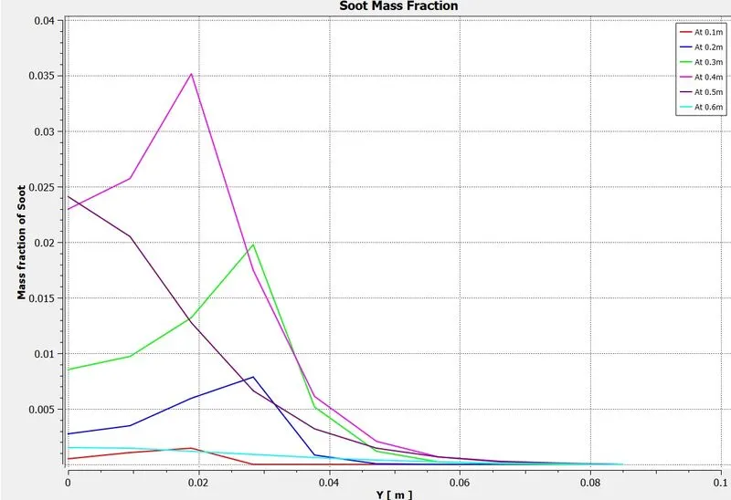
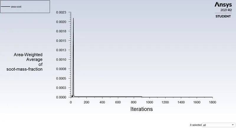
Area Weighted Average of Mass Fraction Of soot At The Outlet -
The value of mass fraction of soot at the outlet is 1.5922792e-05.
Temperature Contour -
Mass Fraction Contour of N2 -
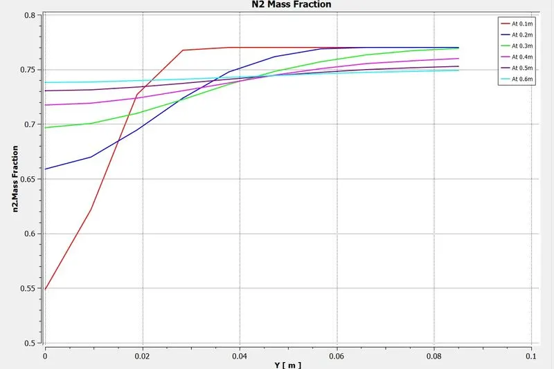
Chart plot showing variation of mass fraction of N2 -
Mass Fraction Contour of H2O -
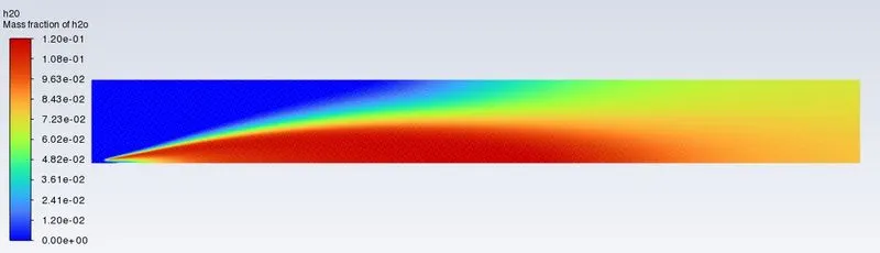
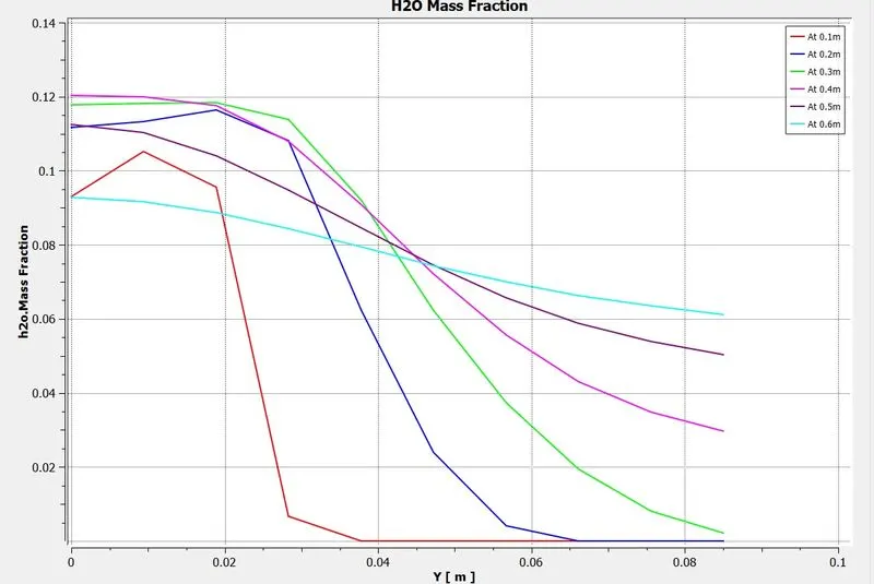
Chart plot showing variation of mass fraction of H2O -
Mass Fraction Contour of CO2 -
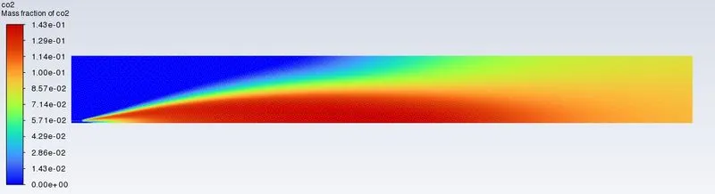
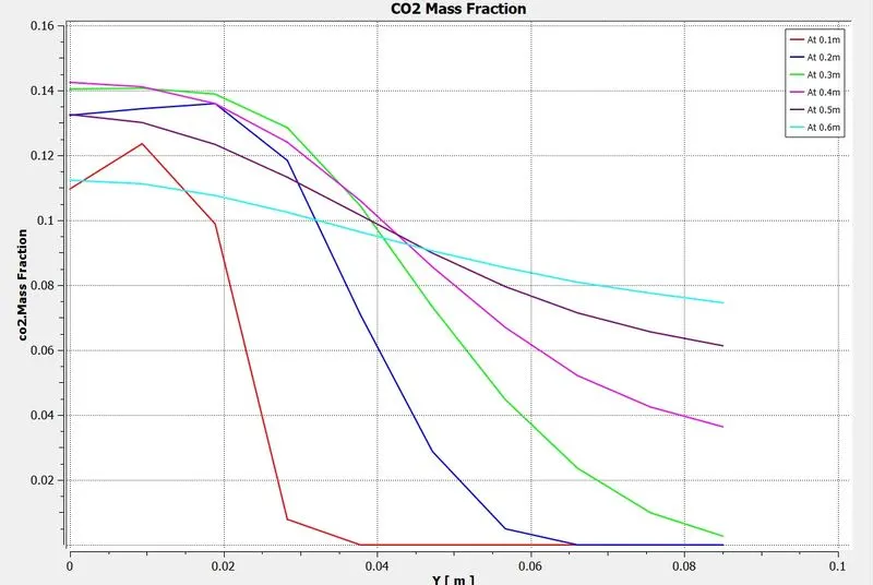
Chart plot showing variation of mass fraction of CO2 -
Mass Fraction Contour of CH4 -
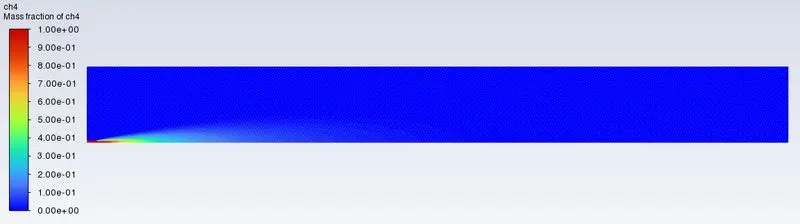
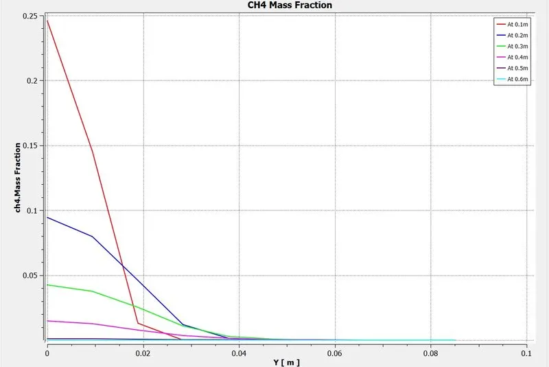
Chart plot showing variation of mass fraction of CH4 -
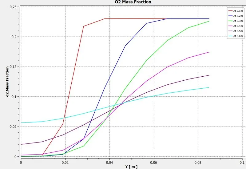
Mass Fraction Contour of O2 -
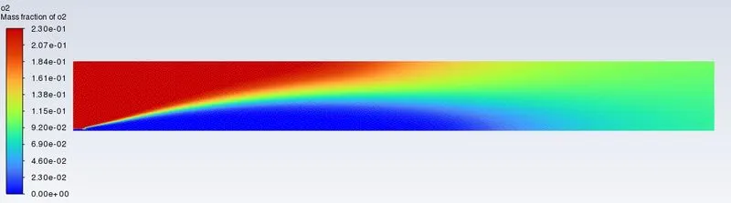
Chart plot showing variation of mass fraction of O2 -
Mass Fraction Contour of NOx -
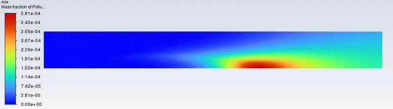
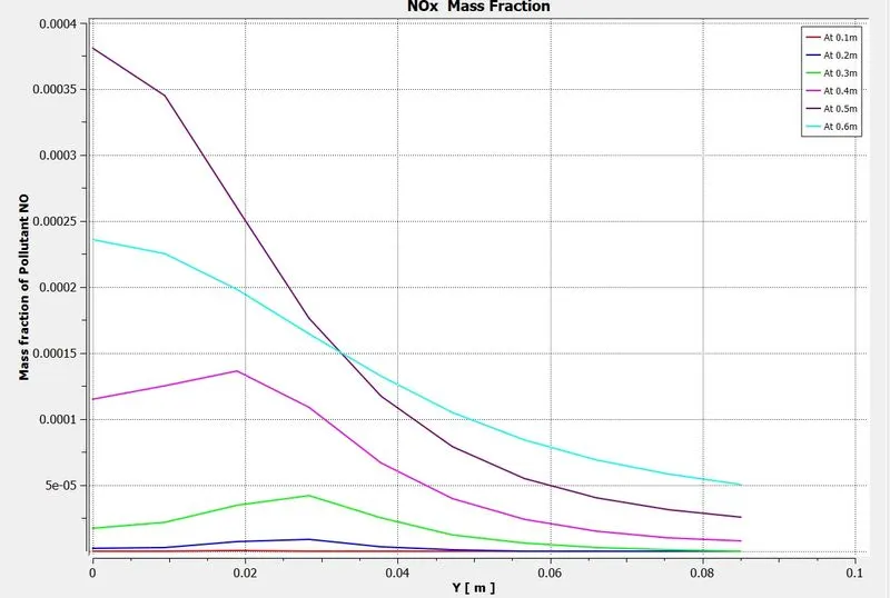
Chart plot showing variation of mass fraction of NOx -
Mass Fraction Contour of soot -
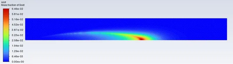
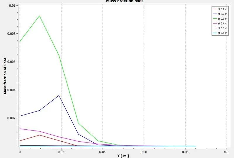
Chart plot showing variation of mass fraction of soot -
5] Part 2 -
*In this part we need to add water content in the fuel from 5% to 30% by mole and observe the effect of it on the result.We
will provide line plots and contours to prove our claim and will use parametrc study approach for this.
*Everything is same from geometry preparation to meshing.
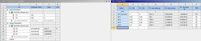
*Since,we are performing parametric study,we need to set input and output parameters which we want to parametrise.
*We will set water and CH4 mass fraction as input parameters and want to keep track of temperature ,mass fraction of Nox and soot at the outlet as output parameters.
*To parametrize mass fraction of H2O and CH4 as input parameters,follow the below steps -
In boundary condition for fuel,under species mass fraction instead of giving values of mass fraction,click on the side options of CH4 and select new input parameter => name it => ok.
*Simillarly set the mass fractions of H2O as new input parameter and for all remaining species give zero.
*Now to parametrize temperature and mass fraction of NOx and soot,
In solutions tab => click definitions => new => surface report => area weighted average => select temperature as field variable and under it as static temperature => in surfaces select outlet => check report file & report plot => to parametrize temperature select the output parameter at the bottom => ok
*Simillarly create prametric report for NOx and soot at the outlet.
*Close fluent and go back to project schematic ,we can see new option has been added at the bottom of the fluent window,named as 'Parameters'.
*Double click on it.We can see on the right hand side a table consisting of design points and there is a empty row there.
*There we can give input mass fractions of H2O and CH4.We will create 4 design points with water content in the fuel from
5% to 30% (mass fraction for H2O as 0,0.05,0.15,0.25,0.3)as there is already 1 design point with H2O percent 0.S
*To view the updated geometry,meshing,solution data,animations,contours etc of newly created design point,click on retain data.
*After updating design points we can see the values for temperature,NOx and soot for each design point.
*To see the individual solution for a perticular design point,right click on it and select set as current.
5.1] Case 2 - Mass Fraction of CH4 = 0.95 & H2O = 0.05
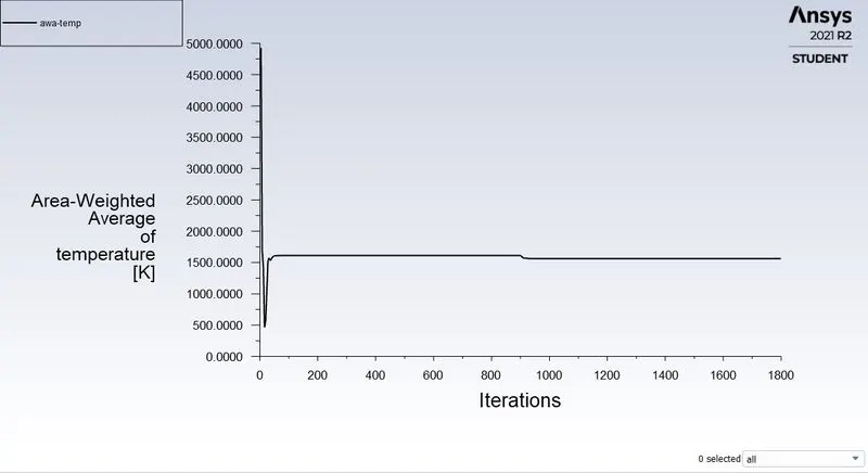
Residual -
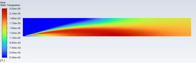
Area Weighted Average of Temperature At The Outlet -
The value of temperature at the outlet is 1561.0247 K.
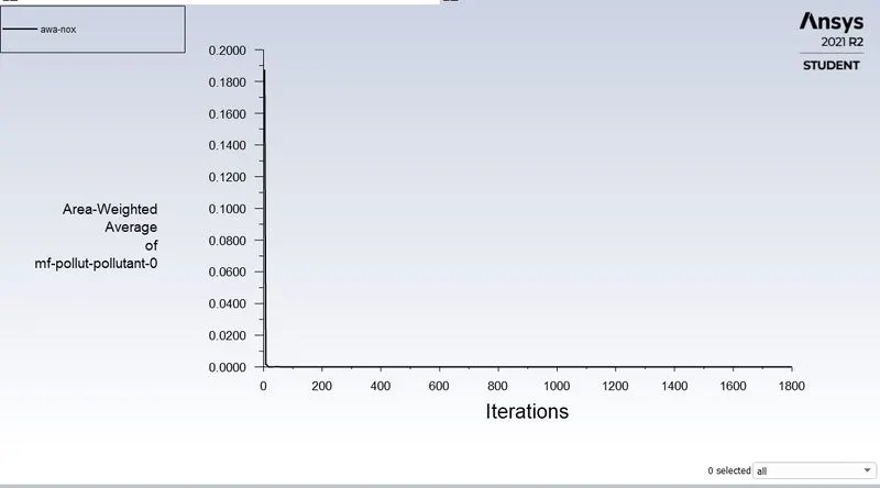
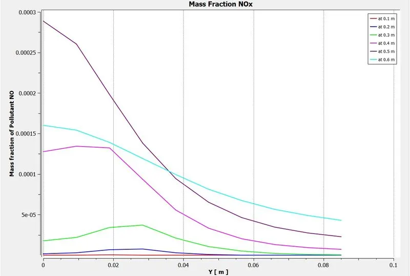
Area Weighted Average of Mass Fraction Of NOx At The Outlet -
The value of mass fraction of NOx at the outlet is 7.814447 e-05.
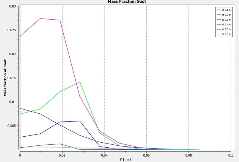
Area Weighted Average of Mass Fraction Of soot At The Outlet -
The value of mass fraction of soot at the outlet is 5.8917186 e-06.
Temperature Contour -
Mass Fraction Contour of N2 -
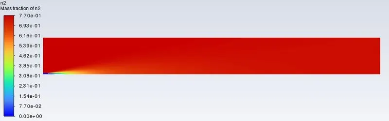
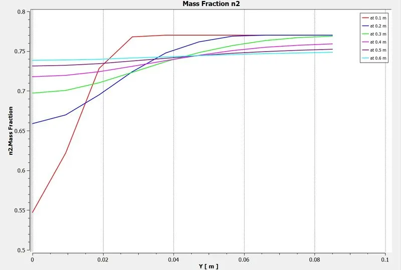
Chart plot showing variation of mass fraction of N2 -
Mass Fraction Contour of H2O -
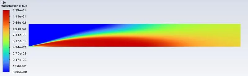
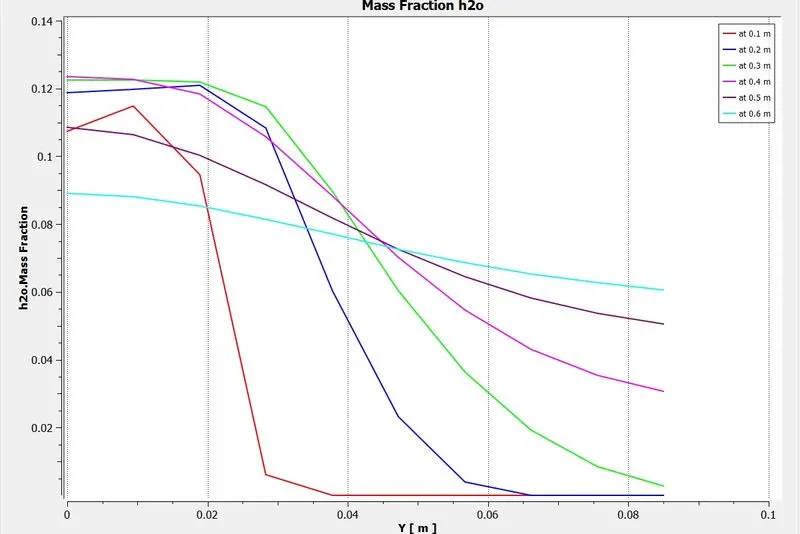
Chart plot showing variation of mass fraction of H2O -
Mass Fraction Contour of CO2 -
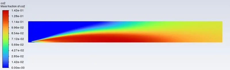
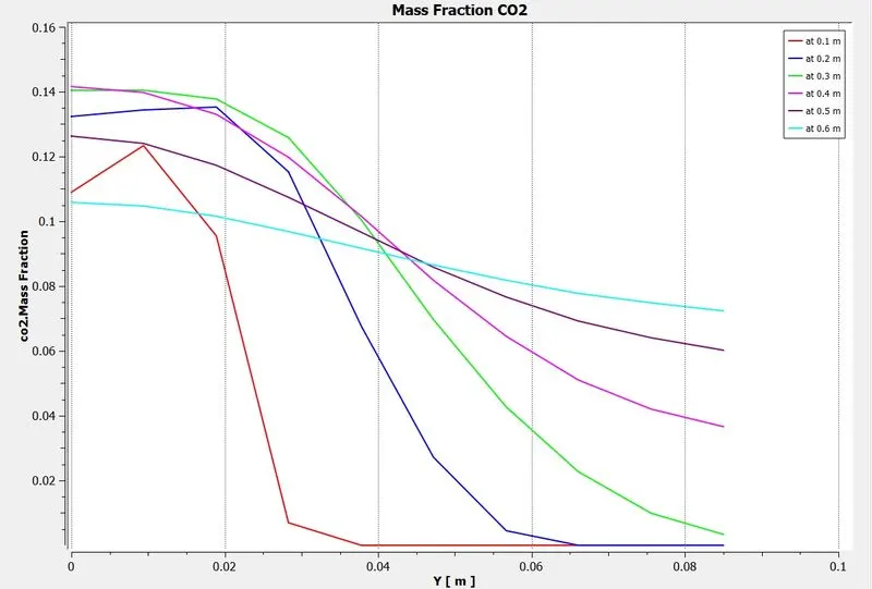
Chart plot showing variation of mass fraction of CO2 -
Mass Fraction Contour of CH4 -
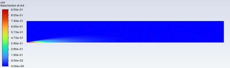
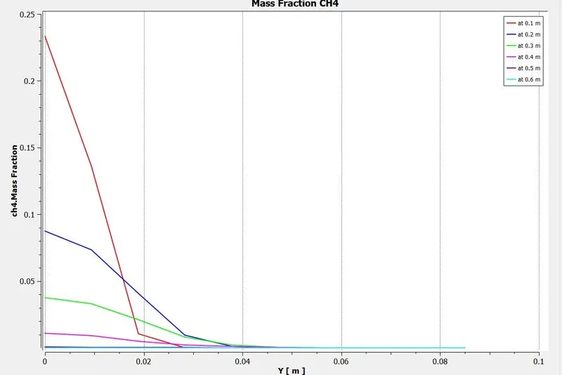
Chart plot showing variation of mass fraction of CH4 -
Mass Fraction Contour of O2 -
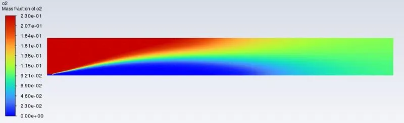
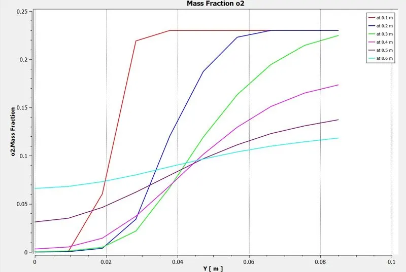
Chart plot showing variation of mass fraction of O2 -
Mass Fraction Contour of NOx -
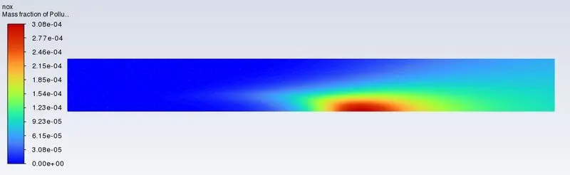
Chart plot showing variation of mass fraction of NOx -
Mass Fraction Contour of soot -
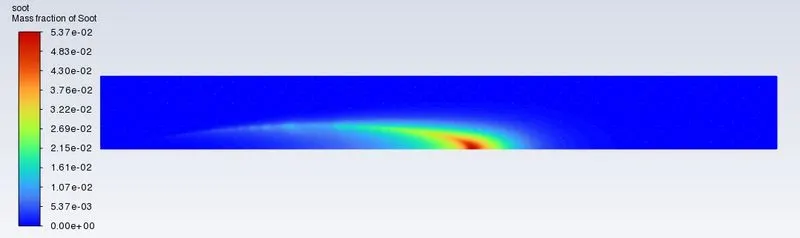
Chart plot showing variation of mass fraction of soot -
5.2] Case 3 - Mass Fraction of CH4 =0.85 & H2O = 0.15
Residual -
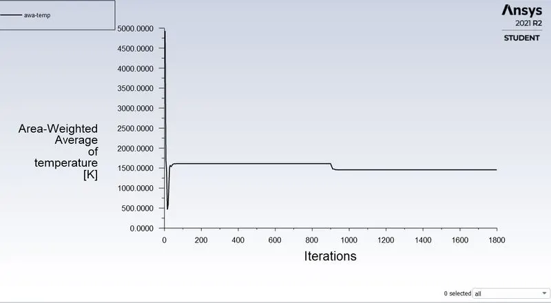
Area Weighted Average of Temperature At The Outlet -
The value of temperature at the outlet is 1456.5 K.
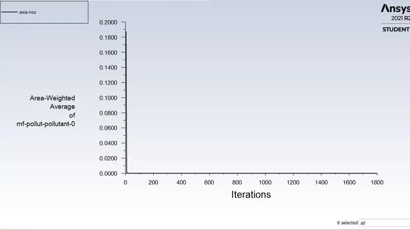
Area Weighted Average of Mass Fraction Of NOx At The Outlet -
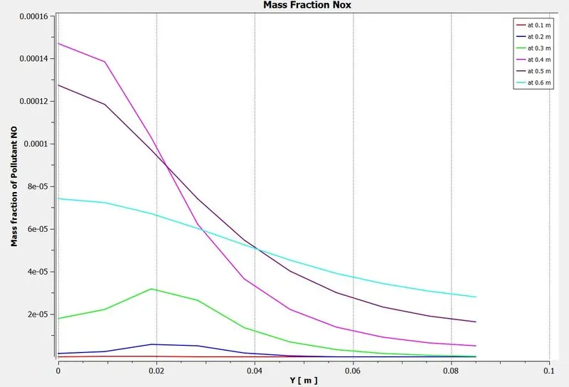
The value of mass fraction of NOx at the outlet is 4.3385 e-05.
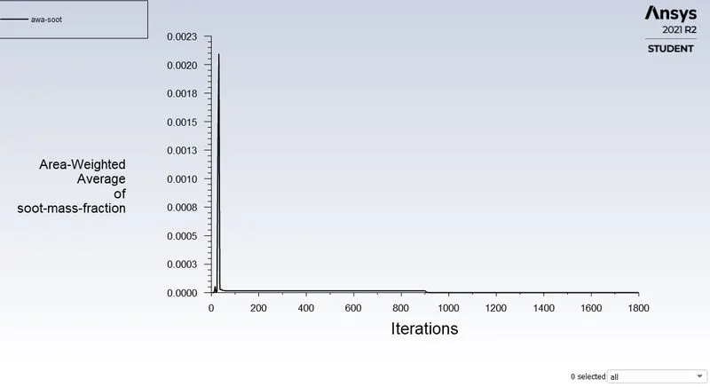
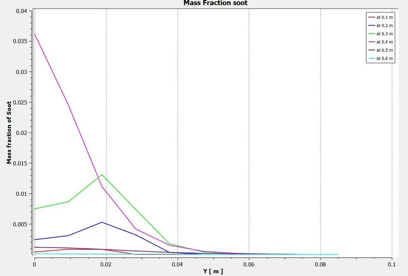
Area Weighted Average of Mass Fraction Of soot At The Outlet -
The value of mass fraction of soot at the outlet is 9.0606 e-07.
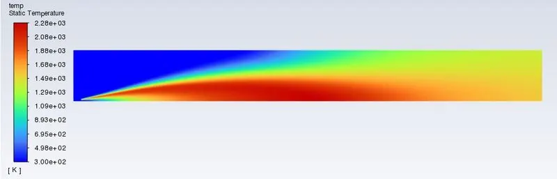
Temperature Contour -
Mass Fraction Contour of N2 -
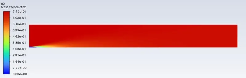
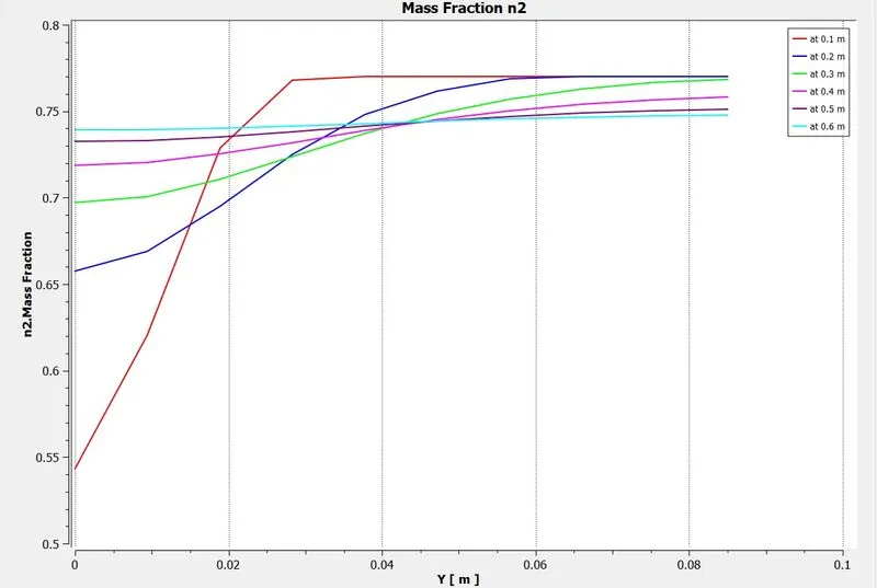
Chart plot showing variation of mass fraction of N2 -
Mass Fraction Contour of H2O -
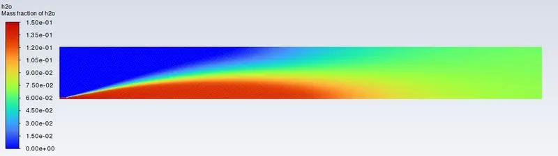
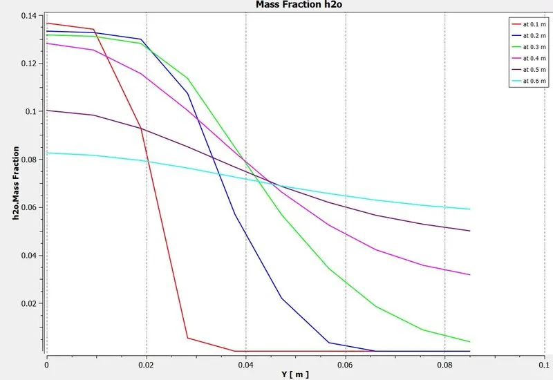
Chart plot showing variation of mass fraction of H2O -
Mass Fraction Contour of CO2 -
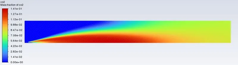
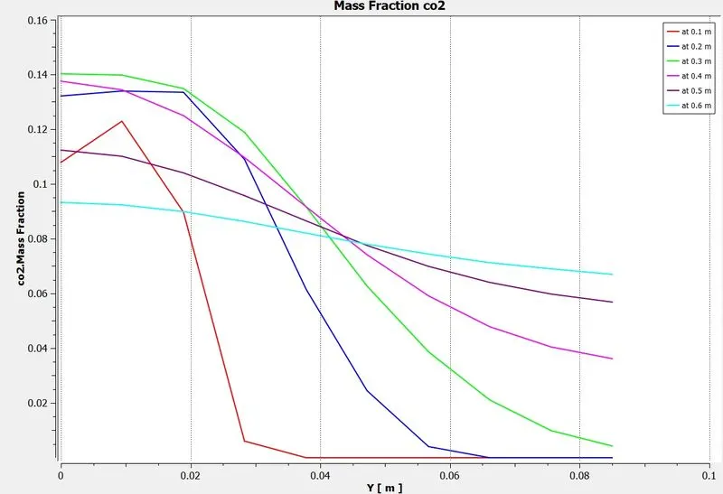
Chart plot showing variation of mass fraction of CO2 -
Mass Fraction Contour of CH4 -
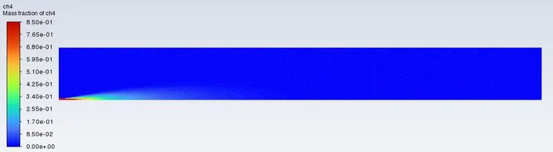
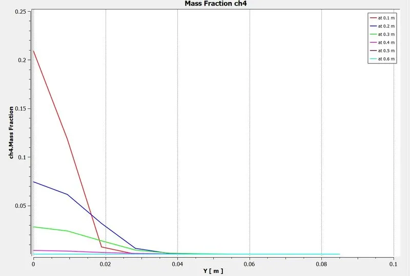
Chart plot showing variation of mass fraction of CH4 -
Mass Fraction Contour of O2 -
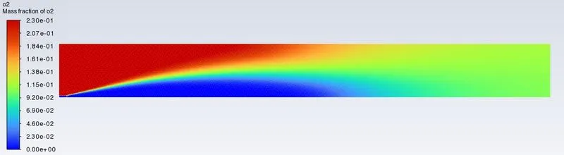
Chart plot showing variation of mass fraction of O2 -
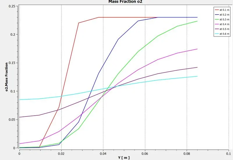
Mass Fraction Contour of NOx -
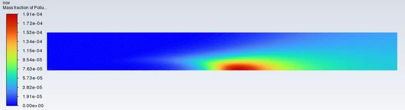
Chart plot showing variation of mass fraction of NOx -
Mass Fraction Contour of soot -
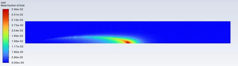
Chart plot showing variation of mass fraction of soot -
5.3] Case 4 - Mass Fraction of CH4 =0.75 & H2O = 0.25
Residual -
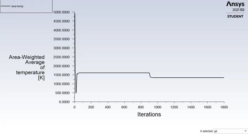
Area Weighted Average of Temperature At The Outlet -
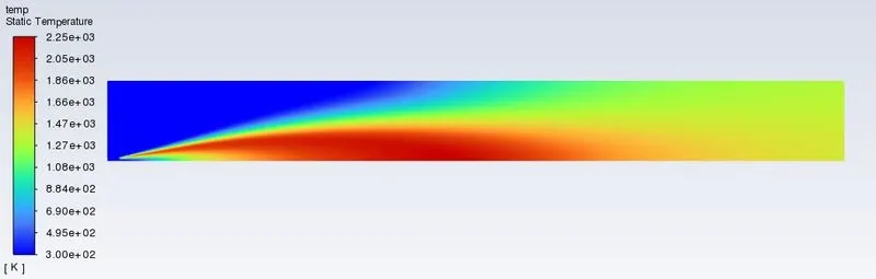
The value of temperature at the outlet is 1347.2 K.
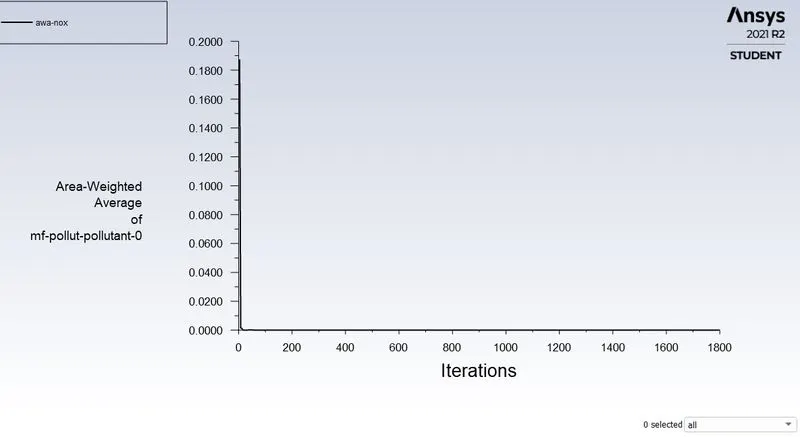
Area Weighted Average of Mass Fraction Of NOx At The Outlet -
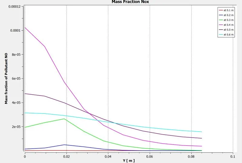
The value of mass fraction of NOx at the outlet is 2.1145 e-05
Area Weighted Average of Mass Fraction Of soot At The Outlet -
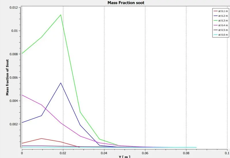
The value of mass fraction of soot at the outlet is 1.0611 e-07.
Temperature Contour -
Mass Fraction Contour of N2 -
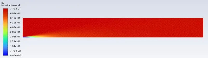
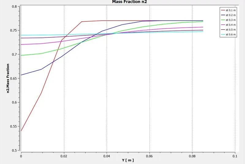
Chart plot showing variation of mass fraction of N2 -
Mass Fraction Contour of H2O -
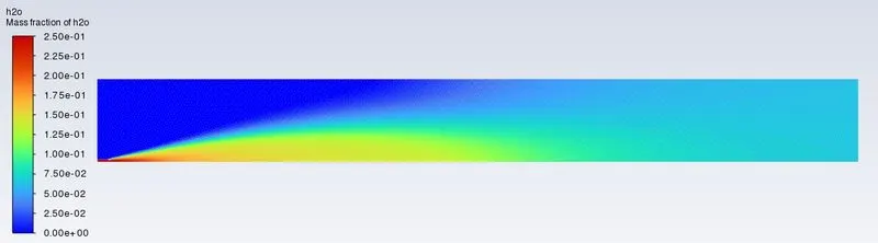
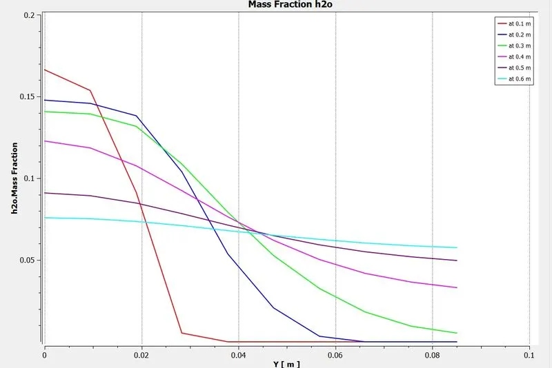
Chart plot showing variation of mass fraction of H2O -
Mass Fraction Contour of CO2 -
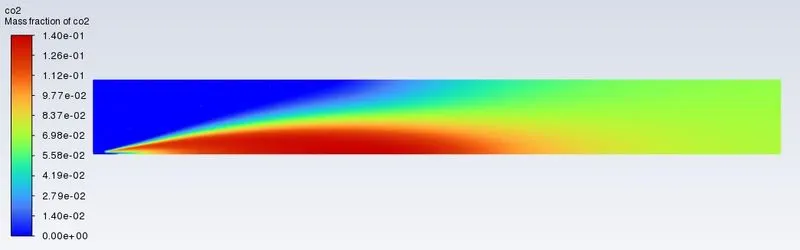
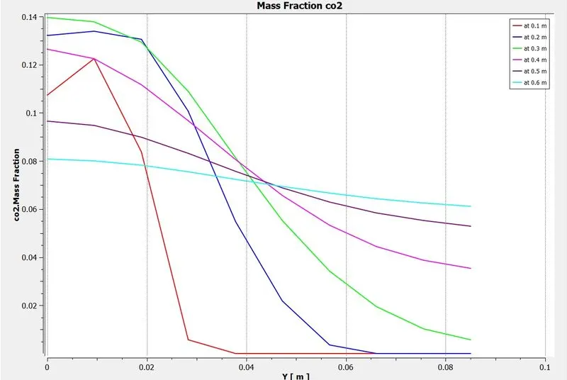
Chart plot showing variation of mass fraction of CO2 -
Mass Fraction Contour of CH4 -
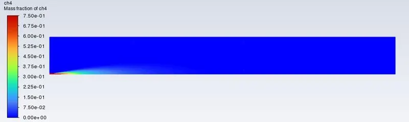
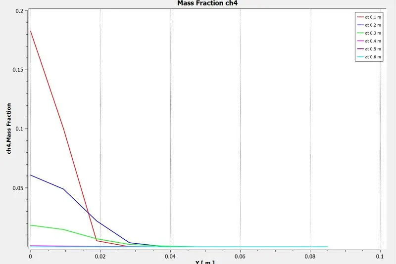
Chart plot showing variation of mass fraction of CH4 -
Mass Fraction Contour of O2 -
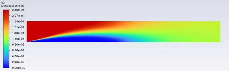
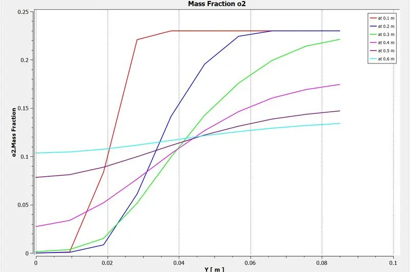
Chart plot showing variation of mass fraction of O2 -
Mass Fraction Contour of NOx -
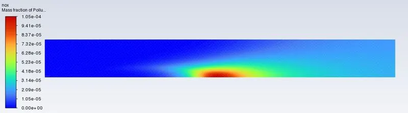
Chart plot showing variation of mass fraction of NOx -
Mass Fraction Contour of soot -
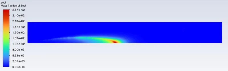
Chart plot showing variation of mass fraction of soot -
5.4] Case 5 - Mass Fraction of CH4 =0.7 & H2O = 0.3
Residual -
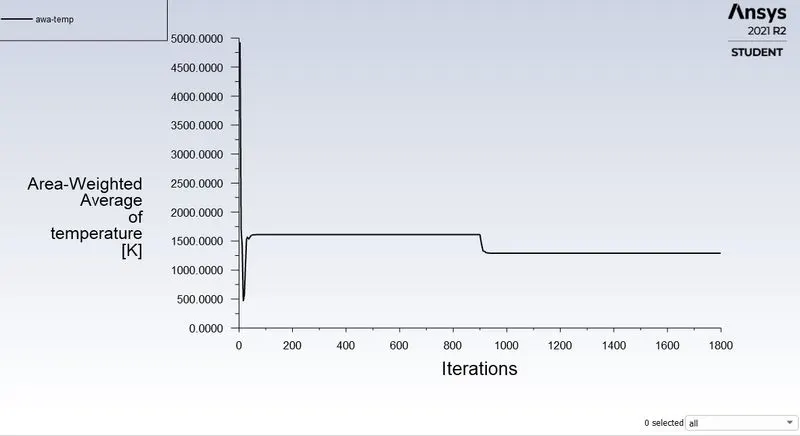
Area Weighted Average of Temperature At The Outlet -
The value of temperature at the outlet is 1290.5 K.
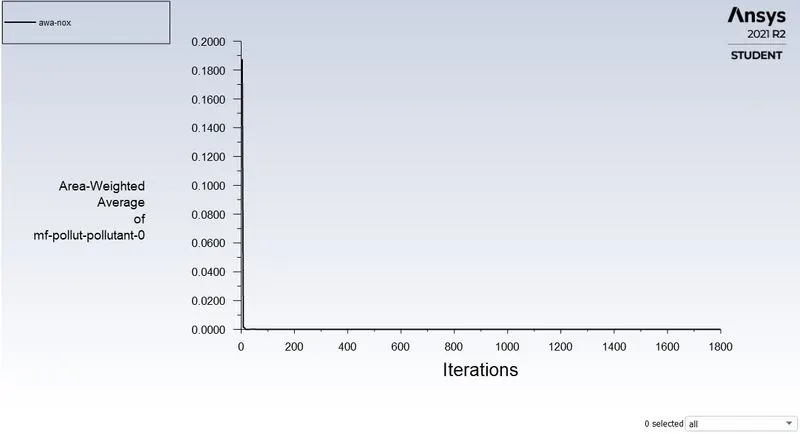
Area Weighted Average of Mass Fraction Of NOx At The Outlet -
The value of mass fraction of NOx at the outlet is 1.3849 e-05.
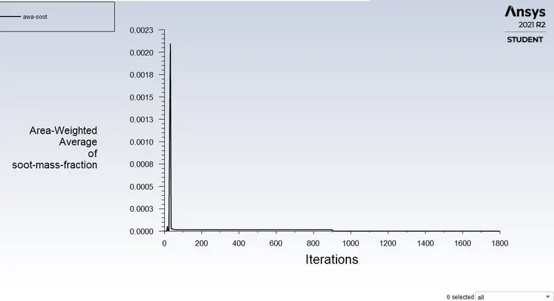
Area Weighted Average of Mass Fraction Of soot At The Outlet -
The value of mass fraction of soot at the outlet is 3.0414 e-08.
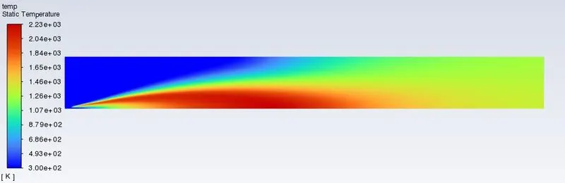
Temperature Contour -
Mass Fraction Contour of N2 -
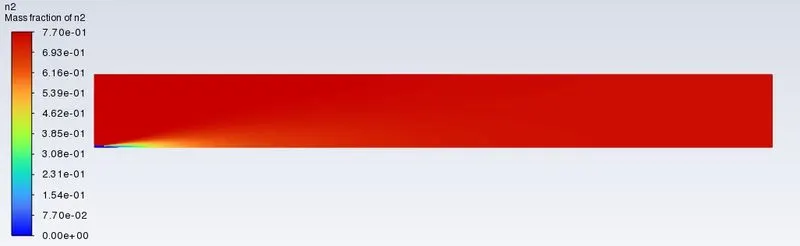
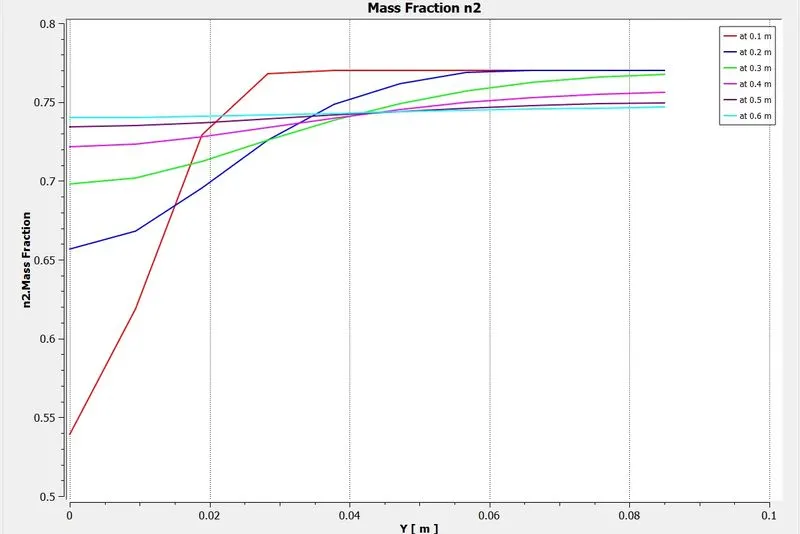
Chart plot showing variation of mass fraction of N2 -
Mass Fraction Contour of H2O -
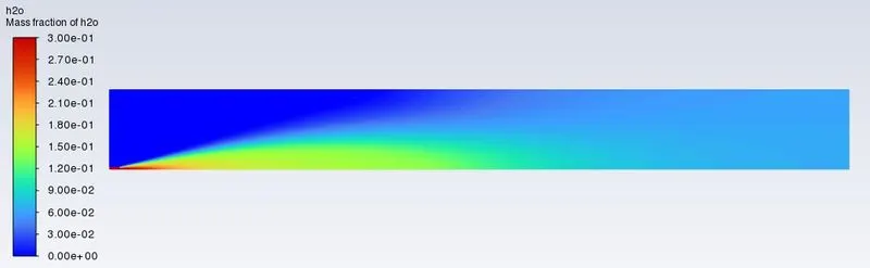
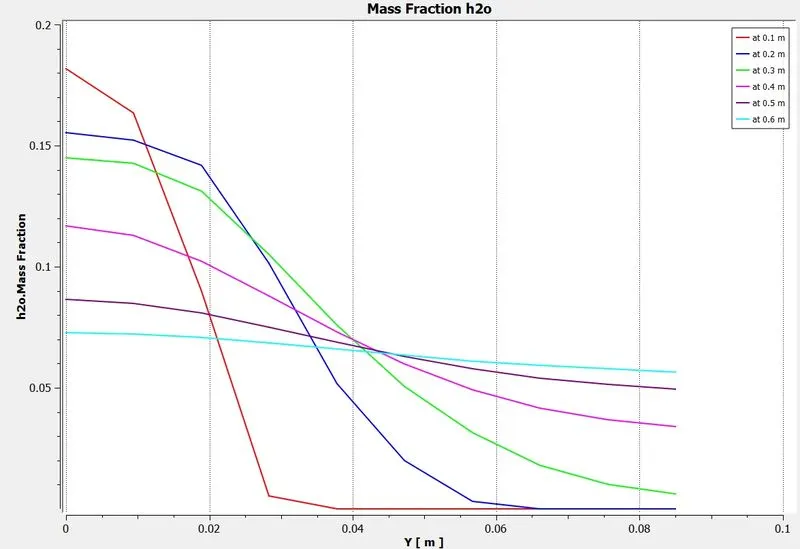
Chart plot showing variation of mass fraction of H2O -
Mass Fraction Contour of CO2 -
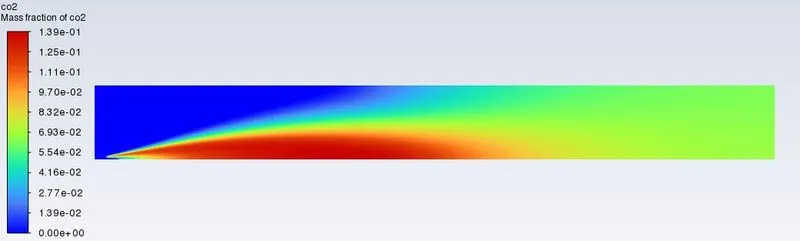
Chart plot showing variation of mass fraction of CO2 -
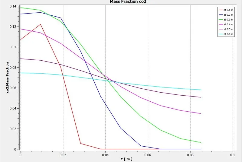
Mass Fraction Contour of CH4 -
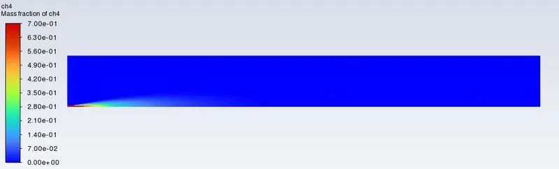
Chart plot showing variation of mass fraction of CH4 -
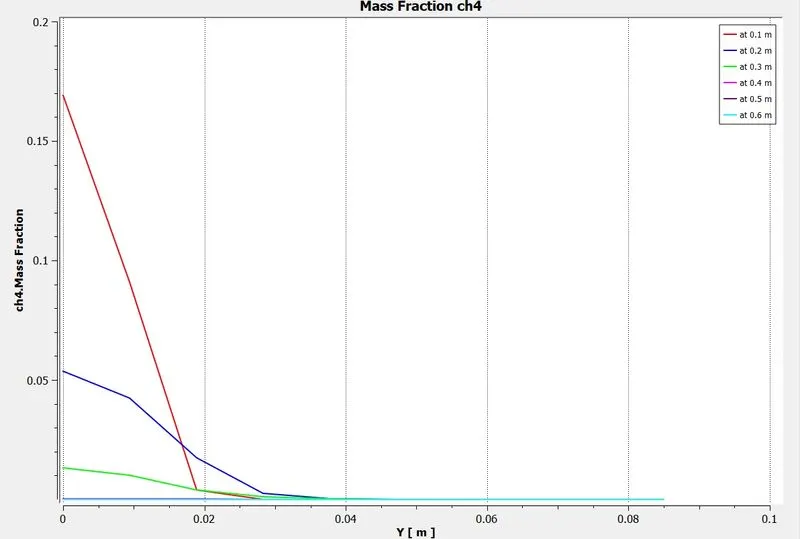
Mass Fraction Contour of O2 -
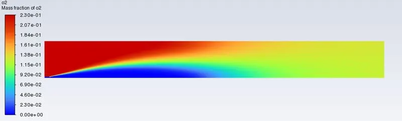
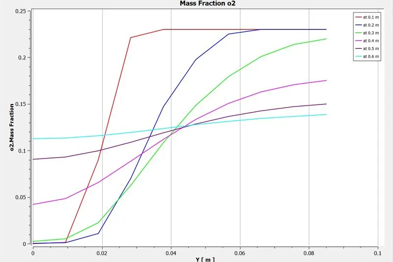
Chart plot showing variation of mass fraction of O2 -
Mass Fraction Contour of NOx -
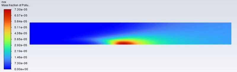
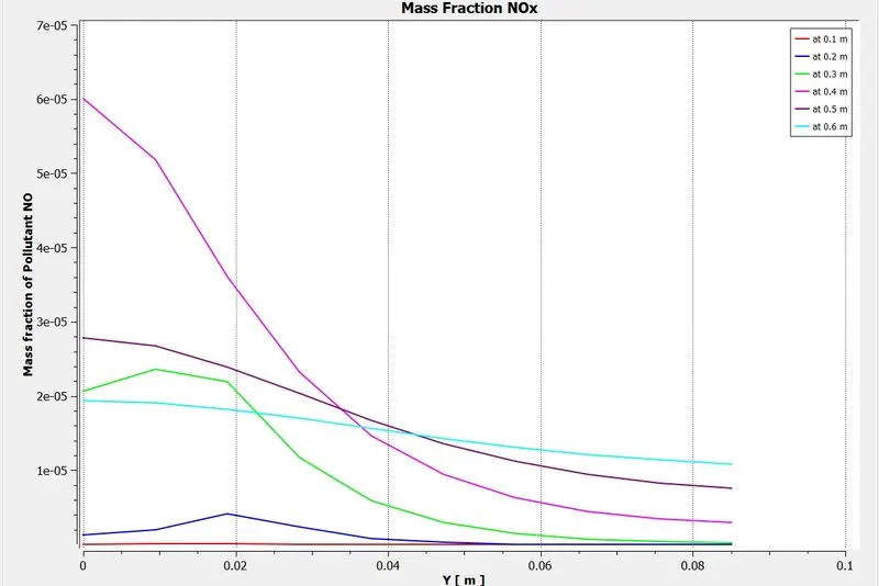
Chart plot showing variation of mass fraction of NOx -
Mass Fraction Contour of soot -
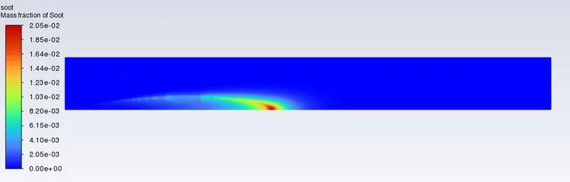
Chart plot showing variation of mass fraction of soot -
| `H_2O%` | `0% H_2O` | `5% H_2O` | `15% H_2O` | `25%H_2O` | `30%H_2O` |
| Temperature(K) | 1611.1809 | 1561.024 | 1456.5 | 1347.2 | 1290.5 |
| Soot | 1.59227 e-05 | 5.8917186 e-06 | 9.0606 e-07 | 1.0611 e-07 | 3.0414 e-08 |
| Nox | 1.020 e-04 | 7.814447 e-05 | 4.3385 e-05 | 2.1145 e-05 | 1.3849 e-05 |
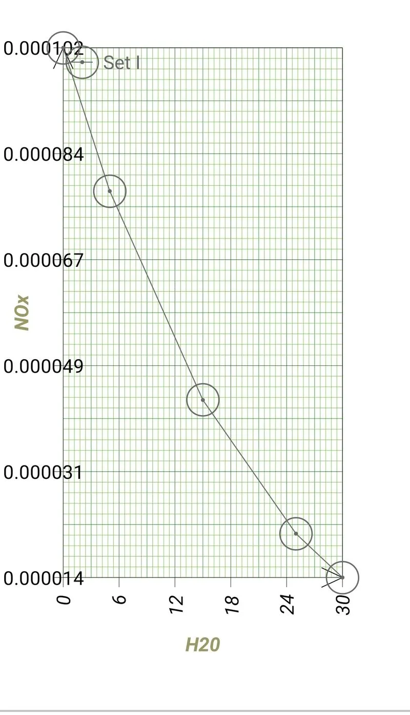
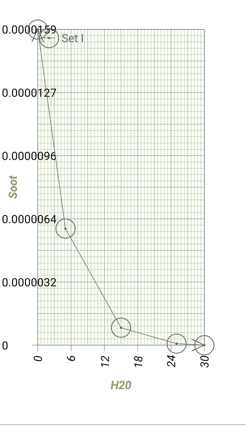
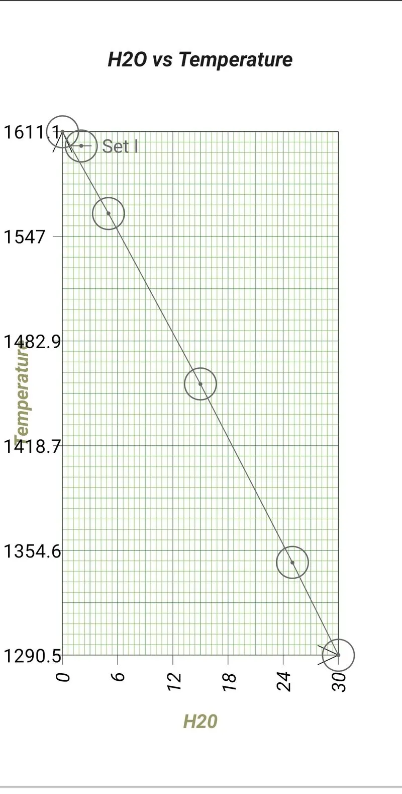
Graph 1 => `H_2O` Vs NOx Graph 2 => `H_2O` Vs Soot Graph 3 => `H_2O` Vs Temperature
6] Conclusion -
*From the above contours and plots we can conclude that adding water to the fuel reduces the emissions.Compairing case 1 and
case 5,we can see that more addition of water the less the emissions.More N2O is formed instead of NO as the temperature decreases.
*But the addition of water causes reduced temperature at the outlet,which in turn causes reduction in efficiency.
*Thermal NOx are temperature dependent while prompt NOx isn't significantly temperature dependent.