Week 1- Mixing Tee
1). Aim -
- Set up steady-state simulations to compare the mixing effectiveness,when the hot inlet temperature is 36C and the cold inlet is 19C.
- Try both k-epsilonand k-omega SST models for the first case to get proper judgement about each method.Later,use the most suitable model for further simulations.
- Simulate each case for the given velocity and momemtum ratio.
- Compare cell count,average outlet temperature,number of iterations for convergence from the 2 cases.
- Plot velocity and temperature contour plots on the cut planes along and across the pipe.
- Also,plot velocity and temperature line plots along and across the length of the pipe.
- Perform Mesh independent study for any one case.
- Discuss the effect of length and momentum ratio on results.
- Later,for each simulation,show the convergence plot
2). Objective -
- Setup Fluent simulation in Ansys workbench.
- Prepare the geometry for simulation,by extracting fluid volume.
- Set up mesh,provide boundary names,give proper element size
- Understand the difference between k-epsilon and k-omega SST turbulence models,and choose the proper model for the given problem.
- Afterward,simulate the problem setup for the number of iterations required to converge our resuts.
- Open results and post-process the simulated data.
- Validate the results by performing a mesh independence study on any one case.
- Study the effect of length and momentum ratio on the results of each case.
- Plot the residual plots to verify ala the results are fully converged after running numerous iterations.
3). Problem Setup -.
We are given 2 cases to simulate the given problem,
Case 1 :
Short Mixing Tee
A) Hot inlet velocity - 3m/s
Momentum ratio - 4
B) Hot inlet velocity - 3m/s
Momentum ratio - 2
Case 2 :
Long Mixing Tee
A) Hot inlet velocity - 3m/s
Momentum ratio - 4
B) Hot inlet velocity - 3m/s
Momentum ratio - 2
3.1) Understanding the difference between k-epsilon and k-omega SST turbulence models,and choosing the proper model for the given problem by considerng case 1(A).
Case 1 :
Short Mixing Tee
A) Hot inlet velocity - 3m/s
Momentum ratio - 4
The k-epsilon and k-omega SST are RANS(Reynolds Averaged Navier Stokes) based turbulence models.k-epsilon models predicts the flow virtually far from the boundaries(wall) and k-omega SST predicts the flow near the walls.Not a single turbulence model suits for every case ,it depends on the need of the specific problem.
In our case to understand which model to use ,we will set two setups for case 1(A) above,one with k-epsilon and another with k-omega SST.The geometry and the mesh will be same for both the setups of case 1(A).
First drag and drop Fluid FLow(Fluent)(this is for k-epsilon) system from toolbox into the project schematic.Then drag and drop another Fluid Flow(Fluent) system(this is for k-omega SST) onto the mesh of the first Fluid FLow(Fluent) system, since we want same mesh and geometry for both setups.
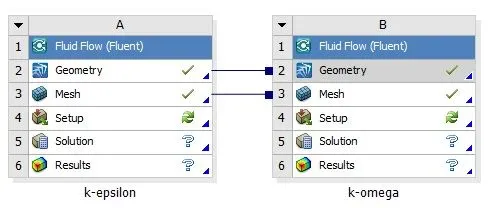
For k-epsilon Method -
3.2) SpaceClaim
Open Ansys SpaceClaim ,set the unit to meters and load the geometry.Extract the fluid volume by using volume extract tool.After,that suppress the solid model for physics,to prevent it from making any conduction.Lastly close the SpaceClaim.
3.3) Mesh
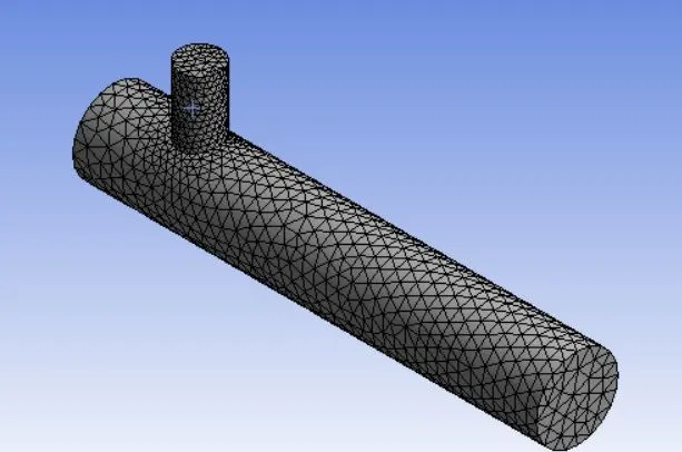
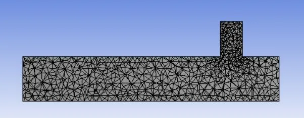
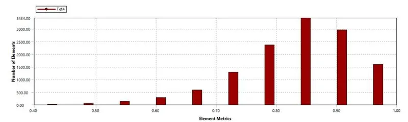
Now,go to meshing, by double cling on mesh,and first do the name selection i.e give proper boundary names.Then generate the basic mesh using generate mesh command.We can see the flow of the mesh inside the extracted volume by using section plane.Also we can check the mesh quality by using mesh quality option.Close the mesh and update it,this will update the mesh for both setups.
3.4) Setup
Double click setup in k-epsilon cell to open Ansys Fluent.The loading of geometry and mesh will start.After successfull loading, we can notice that,Ansys assigned red color to outlet and blue color to inlet.This is the standard practice in Ansys,where red color is assigned to outlet and blue color to inlet.
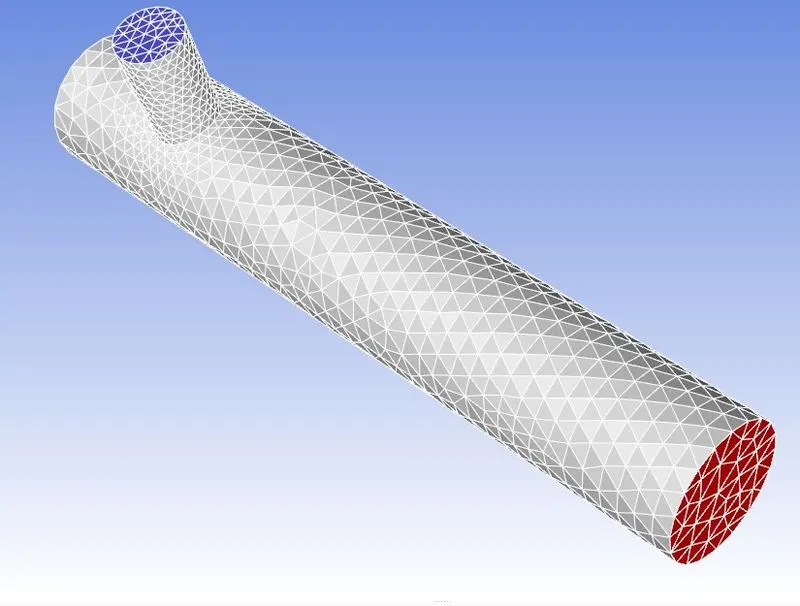
3.4.1) Setting Up Domain :
In setting up the domain,we will first check the mesh to make sure there aren't any mesh discripancies.

3.4.2) Setting up physics :
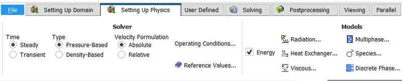
Lets move on to setting up physics.We will be doing steady state simulation of pressure based type.Velocity formulation - Absolute.Next in setting up physics --> models section,turn on the energy equation.This will enable the temperature calculation.
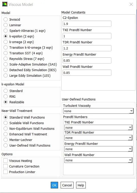
In the viscous model,select 'k-epsilon','realizable'.This is the improved version of k-epsilon model.Keep the remaining settings as default.
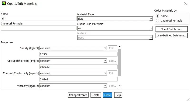
In the materials section keep everything default,as air is our working fluid.We can change that using fluent database option.
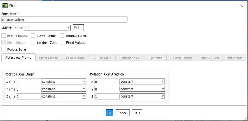
In the cell zones make sure that material is air.
For each boundary do the following changes -
For inlet_x,
Type - velocity-inlet
Velocity Magnitude(m/s) - 3 m/s
Temperature - 36C
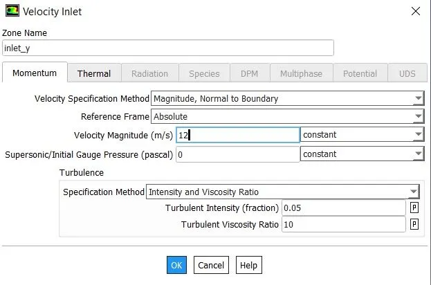
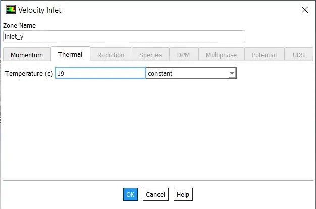
For inlet_y,
Type - velocity-inlet
Velocity Magnitude(m/s) - 12 m/s(Momentum Ratio = 4)
Temperature - 19C
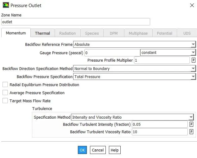
For outlet,
Type - pressure-outlet
Gauge Pressure(pascal) - 0
3.4.3) Solving :
In solving-->Reports,click on defination-->new-->surface report-->area weighted average.Since we want temperature average at outlet surface,select field variable--> temperature,surfaces-->outlet,also check report file and report plot.

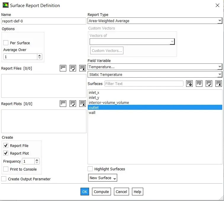
Simillarly,create plot for velocity and create standard deviation plot for temperature.
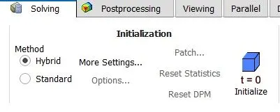
Now we need to initialize our setup.Initialization creates the initial solution that the solver will iterativelly improve.Generally
,the same converged solution is reached,whatever the initialization,though convergence is easier if they are simillar.Basic initialization imposes same values in all cells.
The hybrid initialization method is an efficient method of initializing the solution based purely on the setup of the simulation
with no extra information required.These methods produce a velocity field that conforms to complex domain geometries.After initialization following data gets printed in the console.And calculate for 500 iterations.
********
During calulation we will get converge plot for k-epsilon model.Also report plots for temperature and velocity will get as per our previous setting.
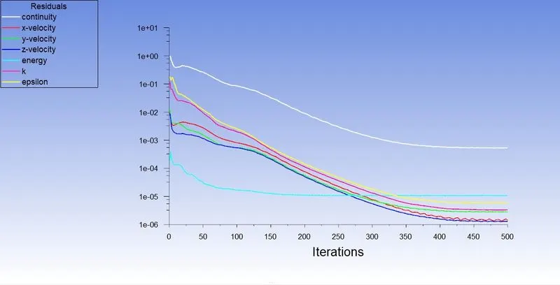
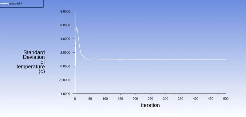
Fig - k-epsilon residual plot Fig - k-epsilon standard deviation of temperature
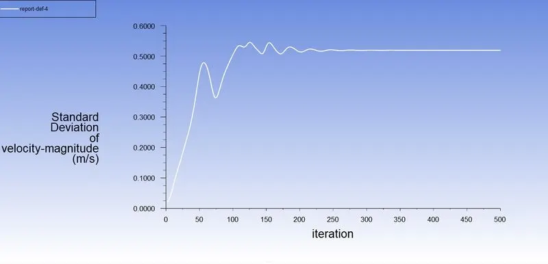
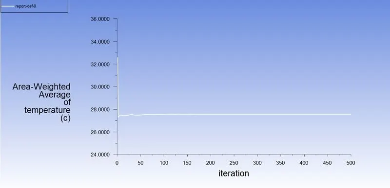
Fig - k-epsilon standard deviation of of velocity magnitude Fig - k-epsilon area weighted average of temperature
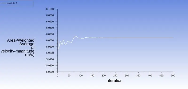
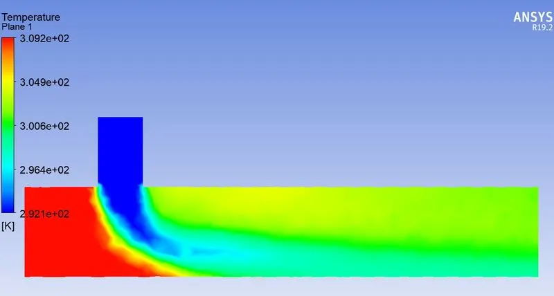
Fig - k-epsilon area weighted average of velocity Fig - k-epsilon temperature contour plot
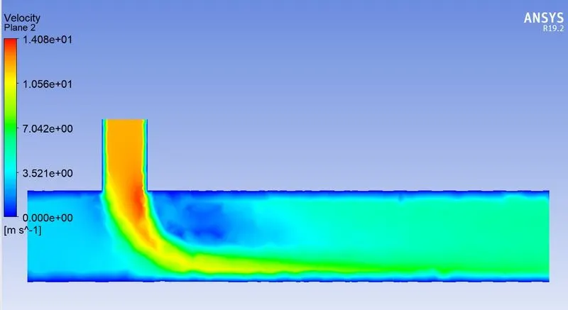
Fig - k-epsilon velocity contour plot
For k-omega SST Method
Follow the same procedure to simulate using k-omega SST and generate plots and compare the results.
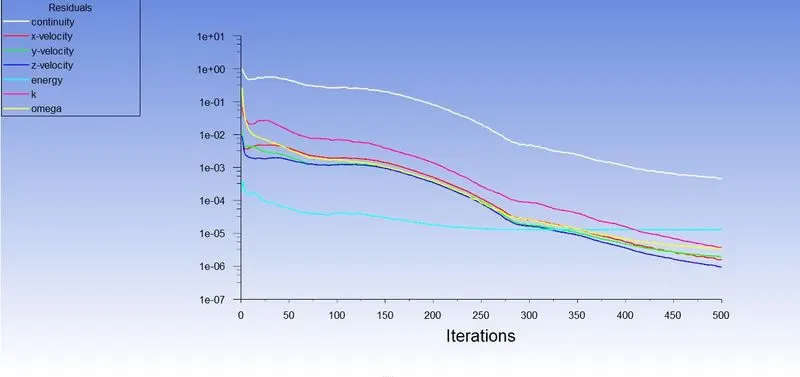
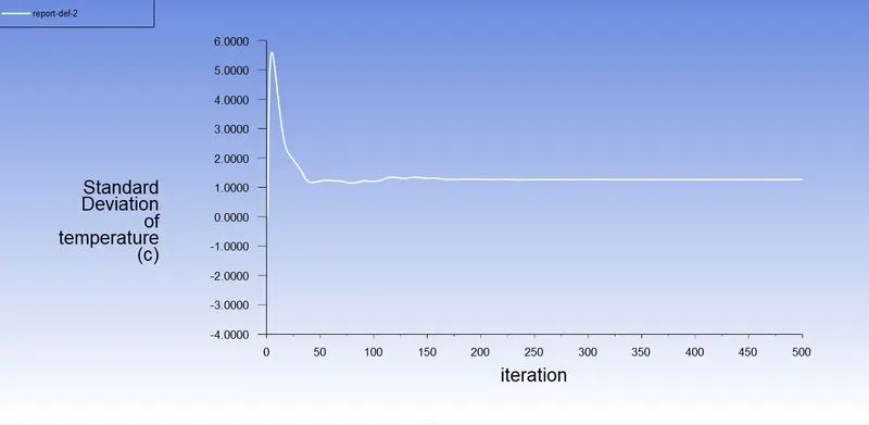
Fig - k-omega residual plot Fig - k-omega standard deviation of temperature
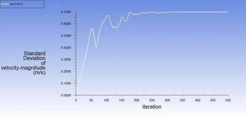
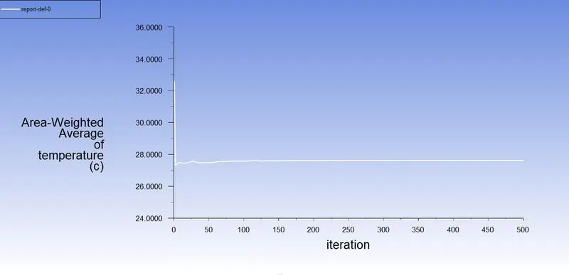
Fig - k-omega standard deviation of of velocity magnitude Fig - k-omega area weighted average of temperature
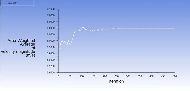
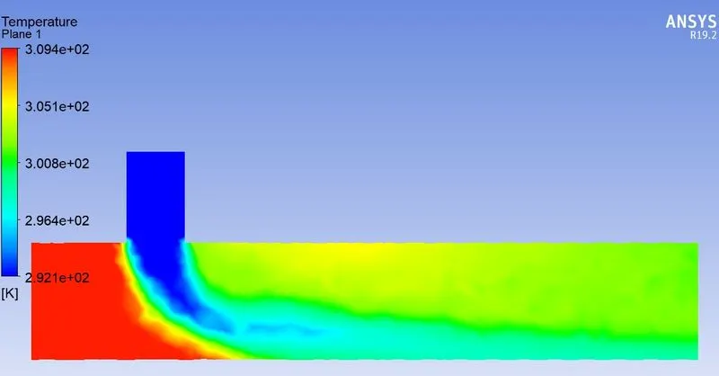
Fig - k-omega area weighted average of velocity Fig - k-omega temperature contour plot
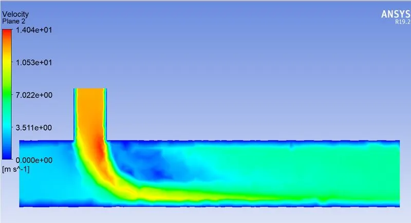
Fig - k-omega velocity contour plot
3.6) Comparing Results And Deciding The Turbulence Model
K-epsilon is the two equation model which gives a description of turbulence by means of two transport equations(PDE).First transported variable is turbulent kinetic energy and second one is the rate of dissipation of turbulent kinetic energy.k-epsilon focuses on the mechanism that affects the turbulent kinetic energy.
On the other hand k-omega SST is a two equation eddy viscosity model,that is mainly used for aerodynamic applications.It's a hybrid model combining the Wilcox k-omega and the k-epsilon modes.A blending function,F1,activates the Wilcox model near the wall and the k-epsilon model in the free stream.This ensures that the appropriate model is utilized through the flow field. k-omega model is best suited for simulating flow in viscous sub-layer.While,k-epsilon model is ideal for predicting flow in the regions away from the wall.The omega model exhibits less sensitivity to free stream conditions than any other turbulece model.The shear stress limiter helps k-omega model avoid a build of excessive turbulent kinetic energy near stagnation points.
Upon observing our simulated figures,we can see that,in the k-omega model flow is more like laminar and not giving proper turbulent results,while simulation by k-epsilon,is giving proper mixing of the two air stream. Since in the given problem we are not dealing with the walls,hence,we are going to use the k-epsilon method for furthere simulations.
4)Simulating given cases with k-epsilon model.
4.1)Short Tee
4.1.1) Inlet Velocity - 3m/s
Momentum Ratio - 4
Cold Air Inlet Velocity -3*4 = 12 m/s
As done above we will share geometry and mesh for momentum ratio = 4 and 2.
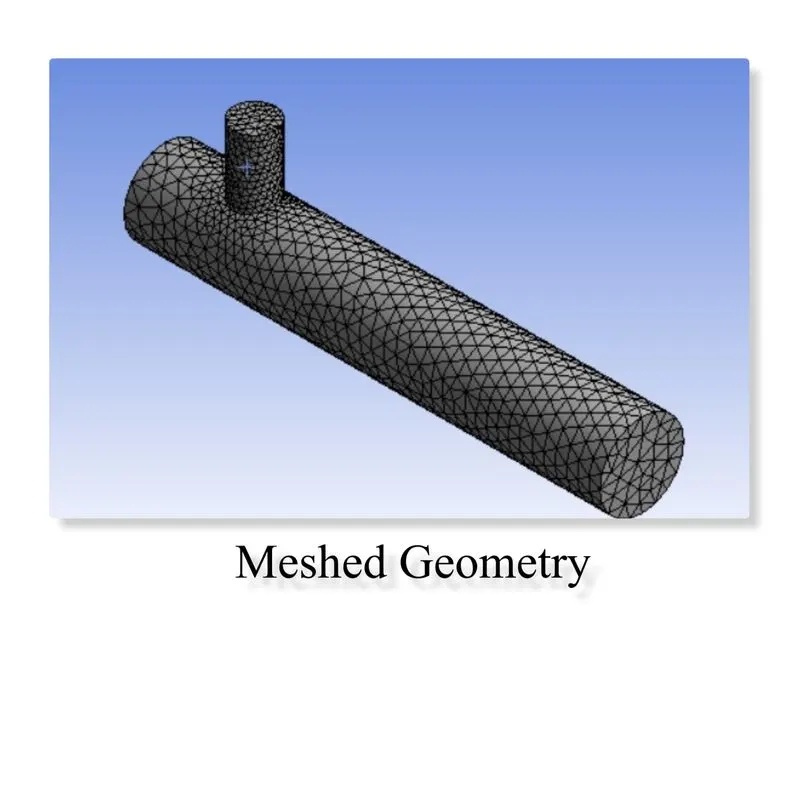
4.1.2) Mesh For Short Tee
In the previous simulation,we can notice,that coarse mesh causing distorted contours near wall surfaces.We can minimise it
by adding inflation layers.
4.1.3)Result
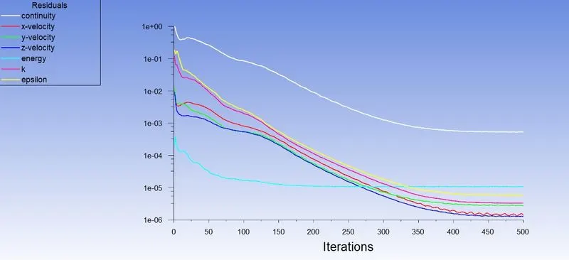
The solution is converging at aroung 425 iterations.
4.1.4) Residual Plot
4.1.5)Temperature
Area weighted average of temperature -
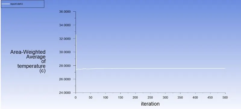
Average temperature at the outlet - 27.487 C
4.1.6)Velocity
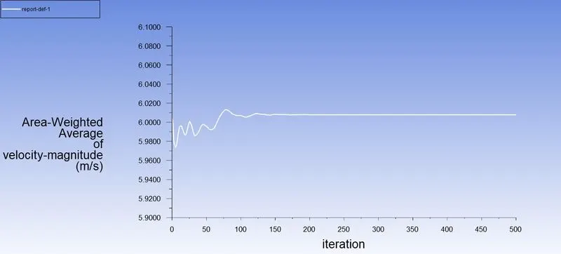
Area weighted average of velocity magnitude -
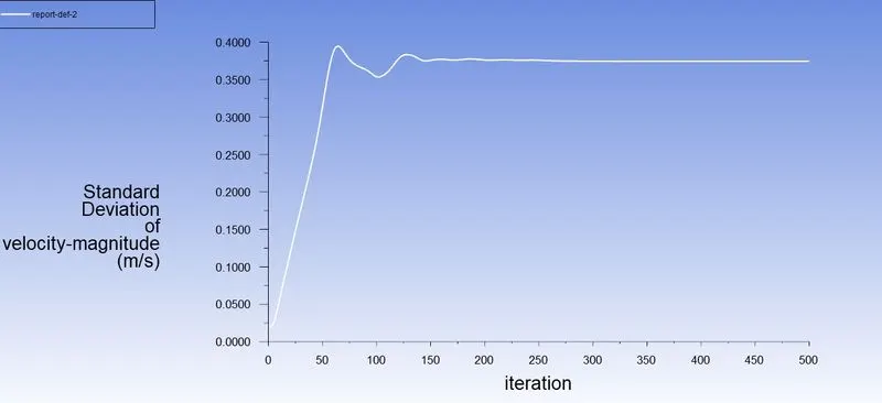
Standard deviation of velocity -
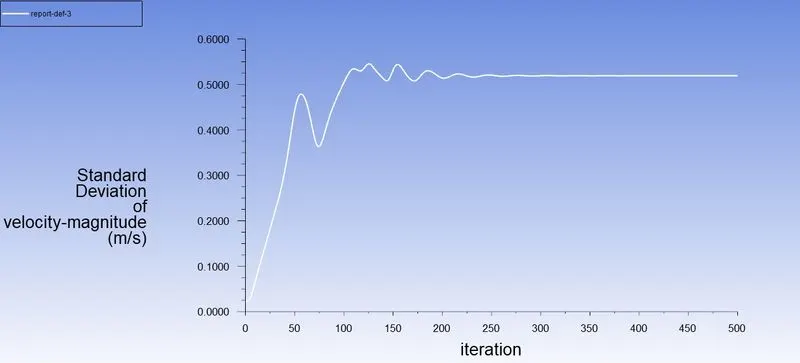
Average velocity at the outlet - 6.027 m/s
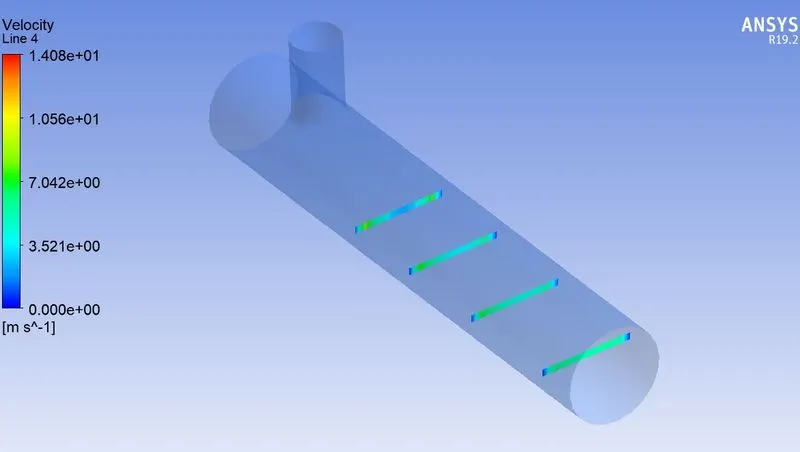
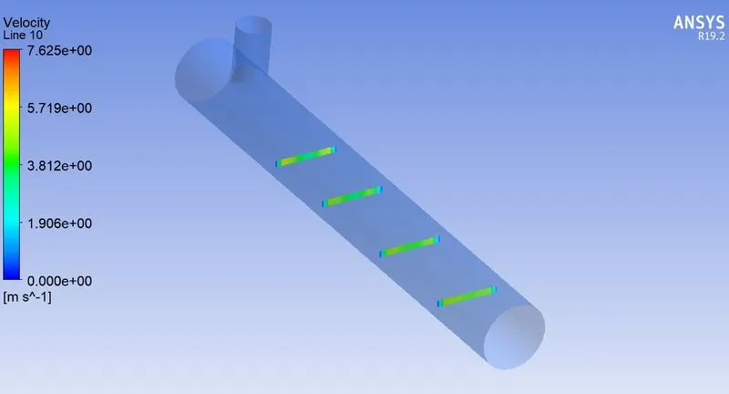
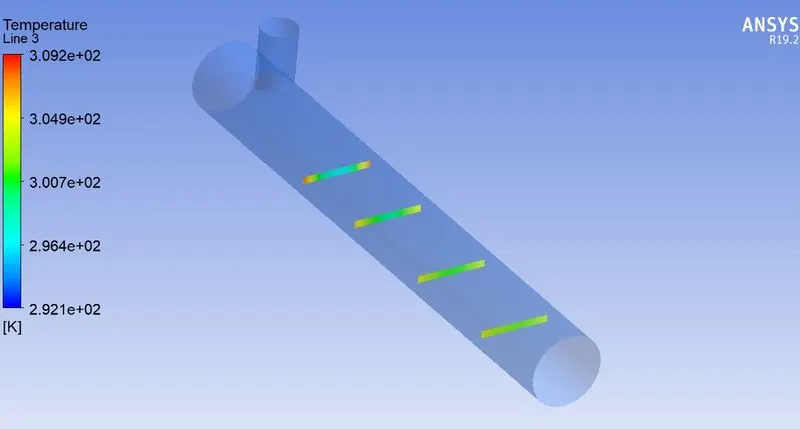
4.1.7)Temperature and velocity contour plots on the cut planes along the pipe
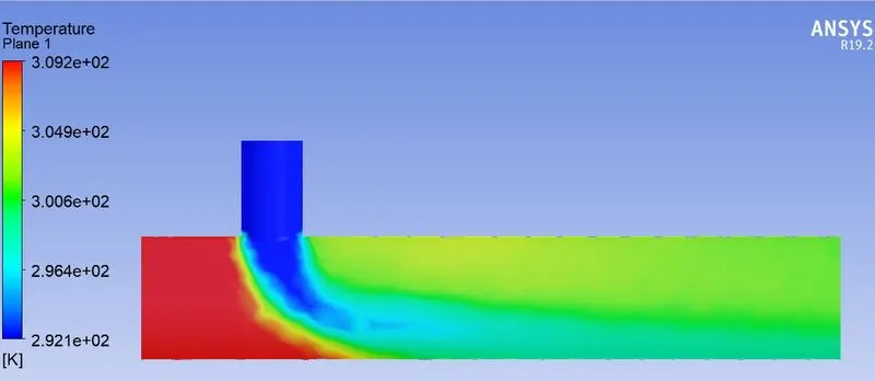
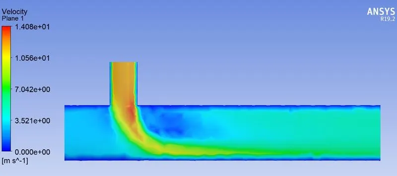
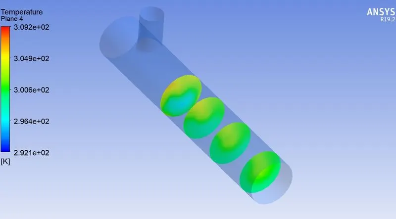
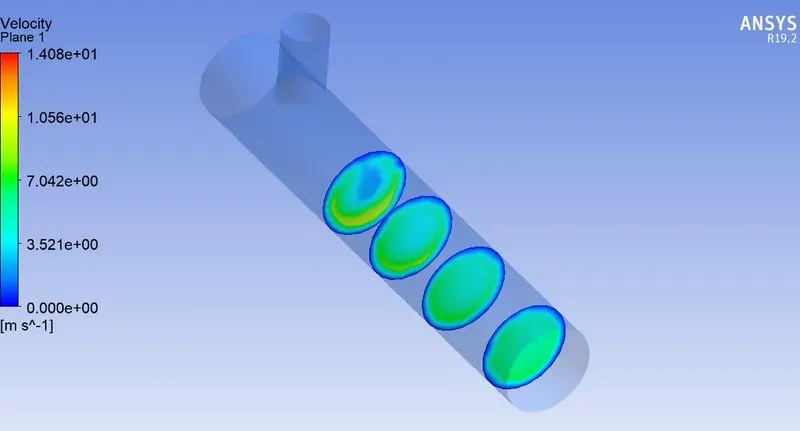
Temperature and velocity contour plots on the cut planes across the pipe
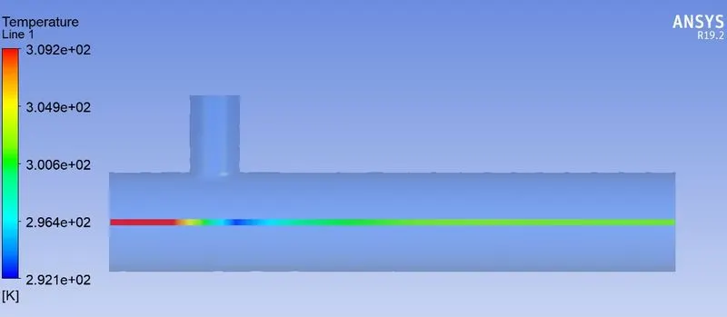
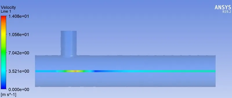
Velocity and temperature line plots along the length of the pipe.
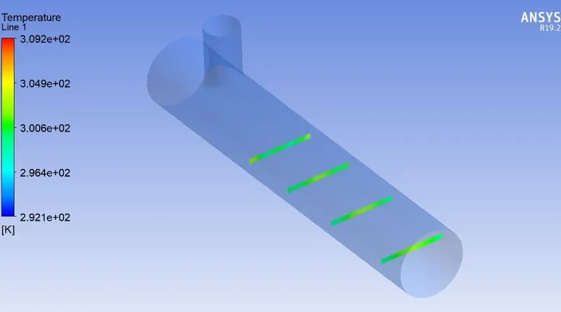
Velocity and temperature line plots across the length of the pipe.
4.1.8) Inlet Velocity - 3m/s
Momentum Ratio - 2
Cold Air Inlet Velocity -3*2 = 6 m/s
4.1.9)Result
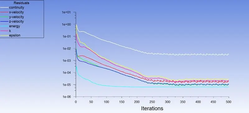
The solution is converging at around 325 iterations.
4.1.10) Residual Plot
4.1.11)Temperature
Area weighted average of temperature -
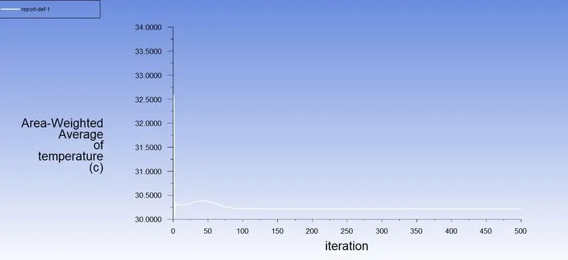
Average temperature at the outlet -30.223 C
4.1.12)Velocity
Area weighted average of velocity magnitude -
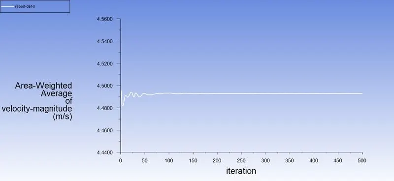
Standard deviation of velocity -
Average velocity at the outlet - 4.504 m/s
4.1.13)Temperature and velocity contour plots on the cut planes along the pipe
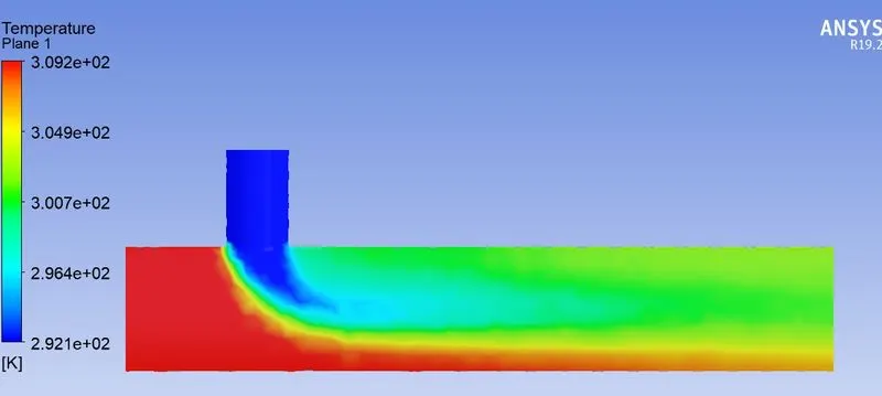
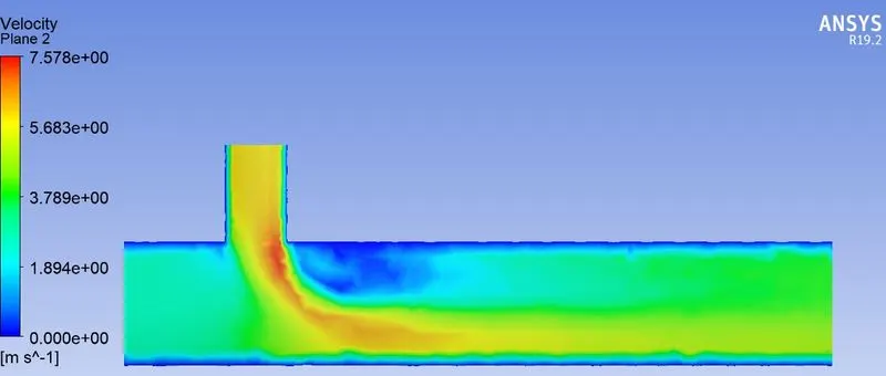
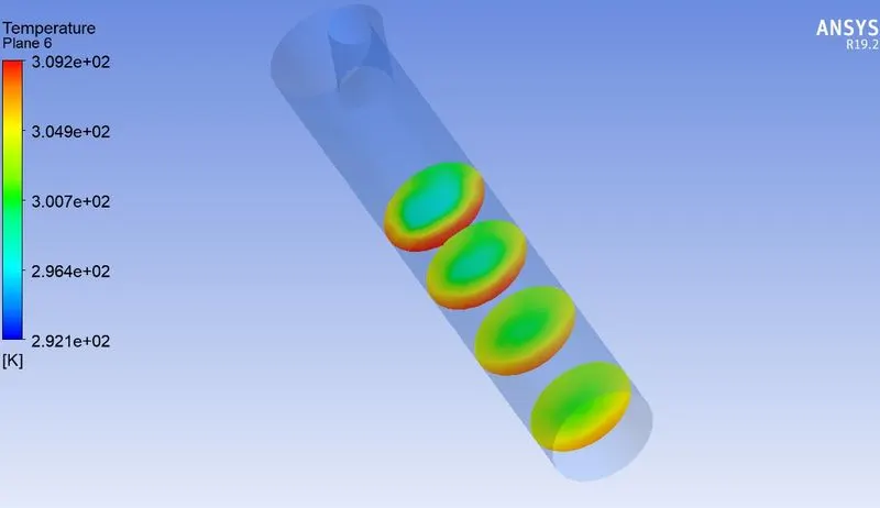
Temperature and velocity contour plots on the cut planes across the pipe
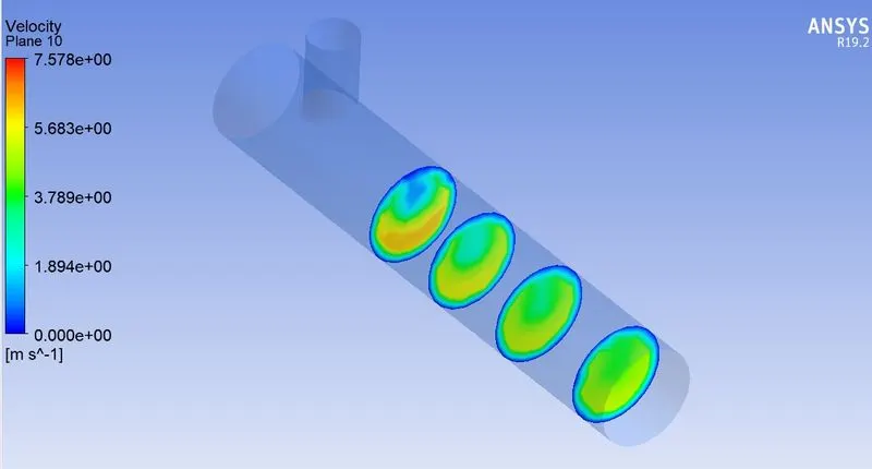
Velocity and temperature line plots along the length of the pipe.
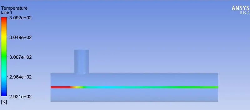
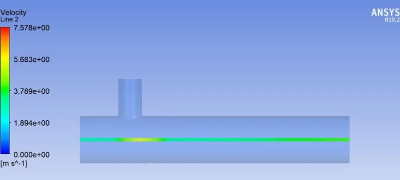
Velocity and temperature line plots across the length of the pipe.
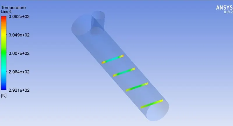
4.2)Long Tee
4.2.1) Inlet Velocity - 3m/s
Momentum Ratio - 4
Cold Air Inlet Velocity -3*4 = 12 m/s
As done above we will share geometry and mesh for momentum ratio = 4 and 2.
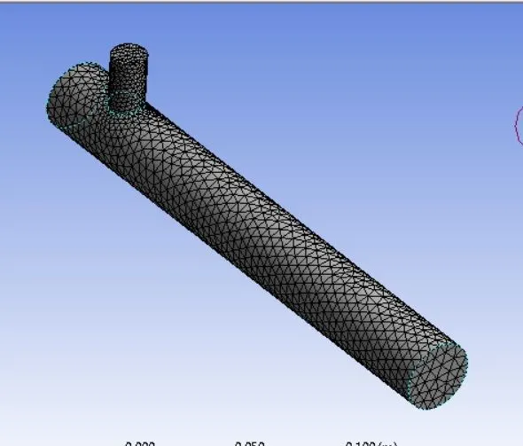
4.2.2) Mesh For Long Tee
In the previous simulation,we can notice,that coarse mesh causing distorted contours near wall surfaces.We can minimise it
by adding inflation layers.
4.2.3)Result
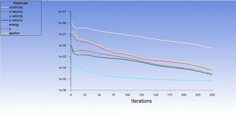
The solution is converging at around 230 iterations.
4.2.4) Residual Plot
4.2.5)Temperature
Area weighted average of temperature -
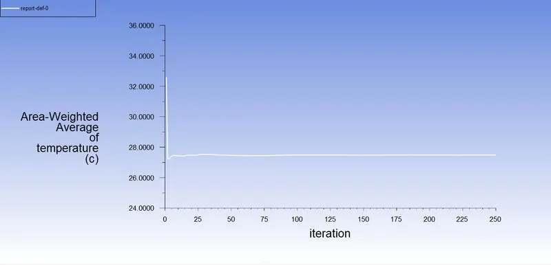
Average temperature at the outlet - 27.481 C
4.2.6)Velocity
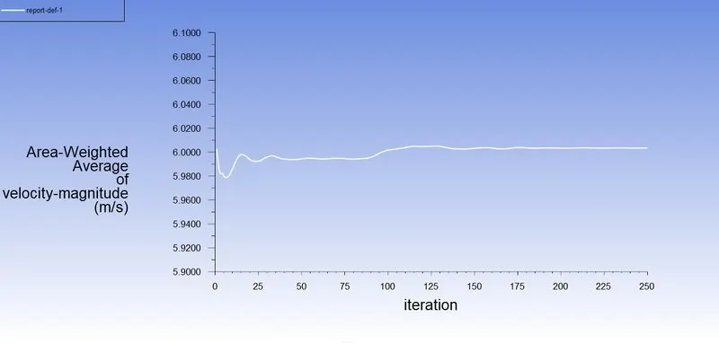
Area weighted average of velocity magnitude -
Standard deviation of velocity -
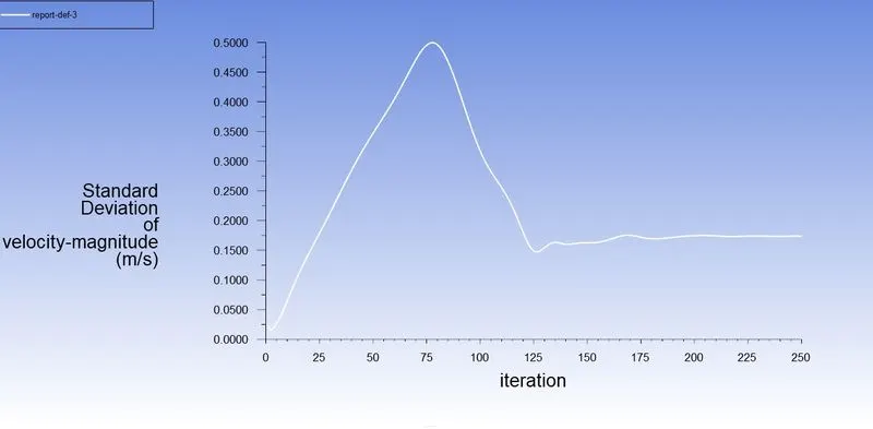
Average velocity at the outlet - 6.003 m/s
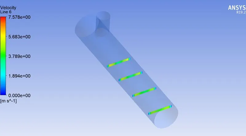
4.2.7)Temperature and velocity contour plots on the cut planes along the pipe
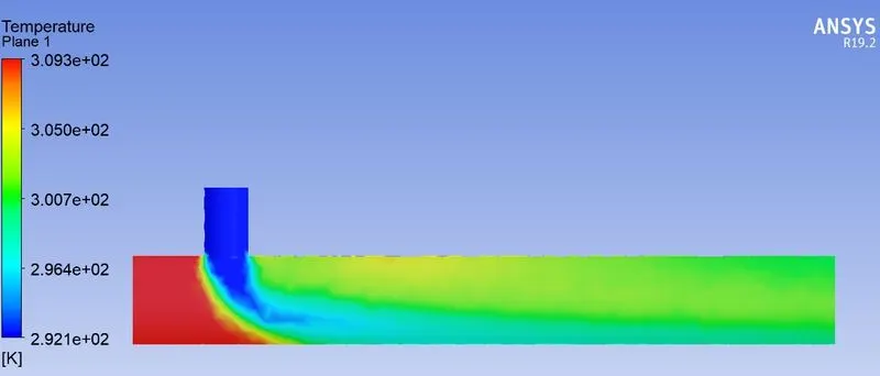
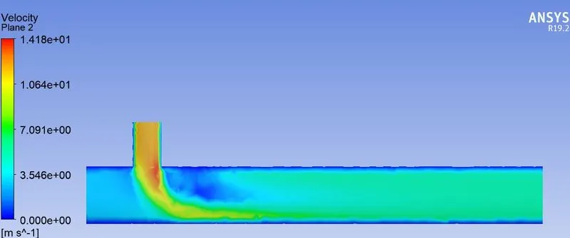
Temperature and velocity contour plots on the cut planes across the pipe
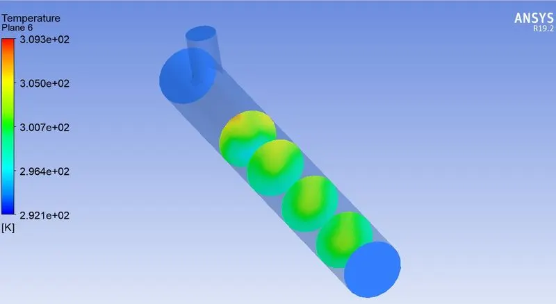
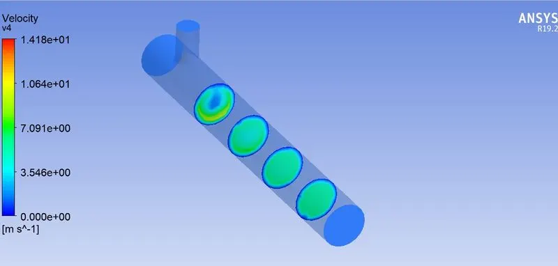
Velocity and temperature line plots along the length of the pipe.
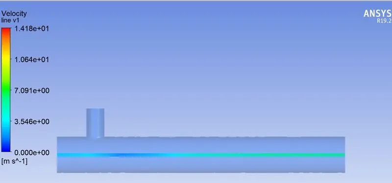
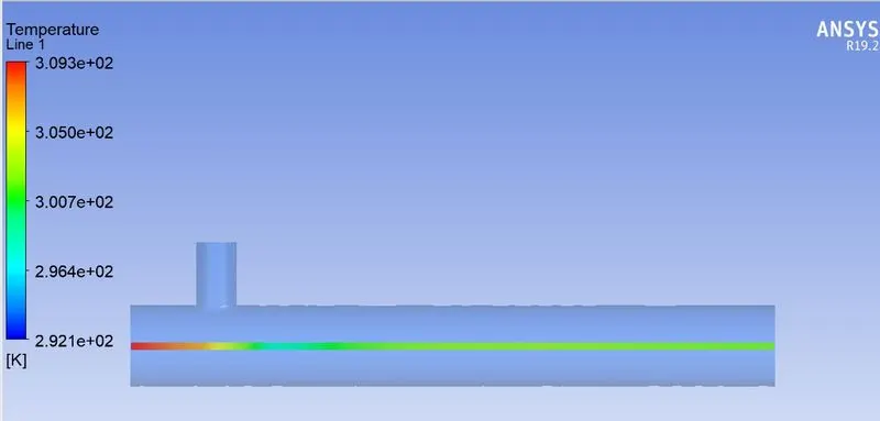
Velocity and temperature line plots across the length of the pipe.
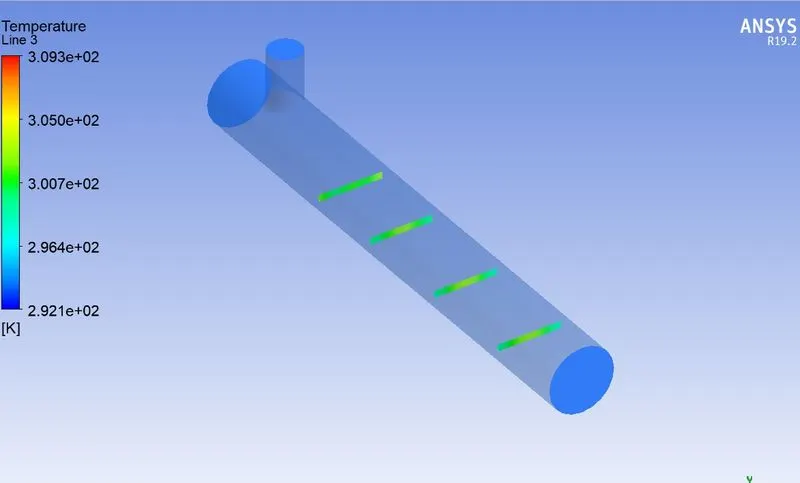
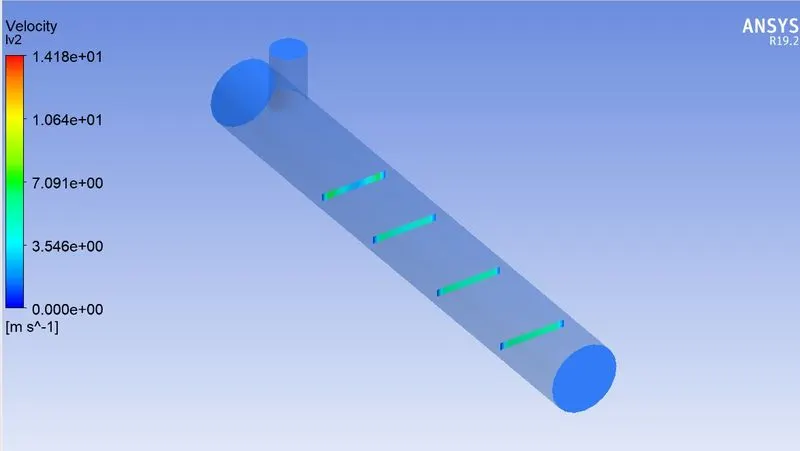
4.2.8) Inlet Velocity - 3m/s
Momentum Ratio - 2
Cold Air Inlet Velocity -3*2 = 6 m/s
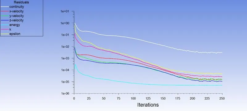
4.2.9)Result
The solution is converging at around 225 iterations.
4.2.10) Residual Plot
4.2.11)Temperature
Area weighted average of temperature -
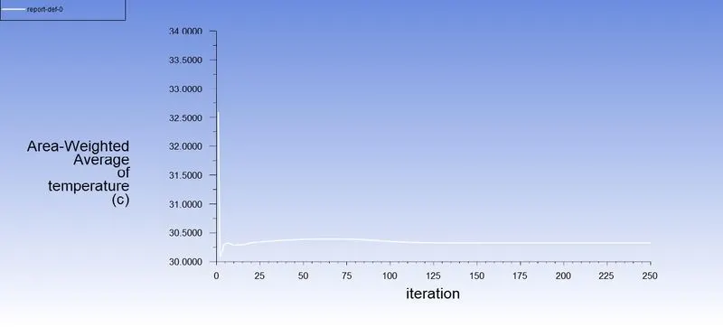
Average temperature at the outlet - 30.320 C
4.2.12)Velocity
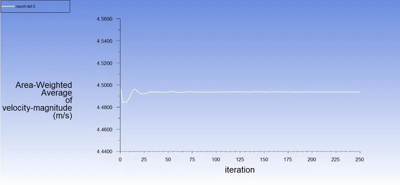
Area weighted average of velocity magnitude -
Standard deviation of velocity -
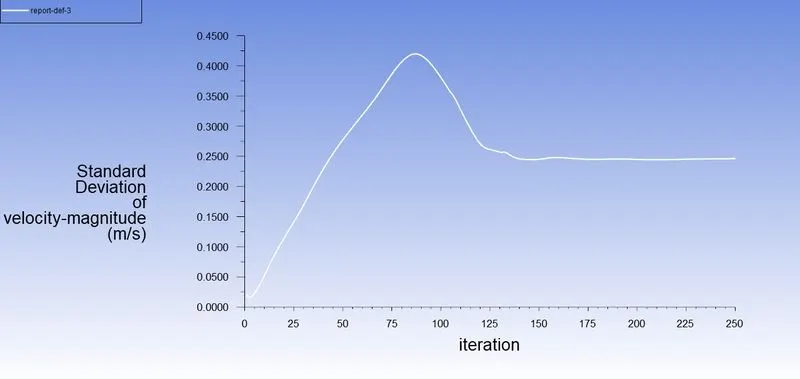
Average velocity at the outlet - 4.493 m/s
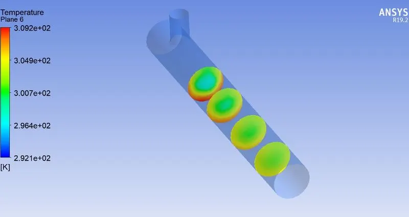
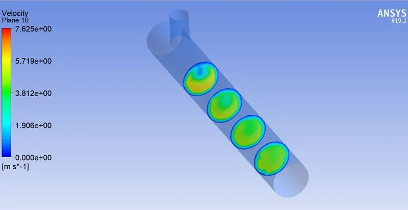
4.2.13)Temperature and velocity contour plots on the cut planes along the pipe
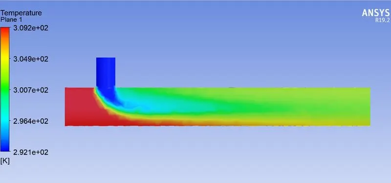
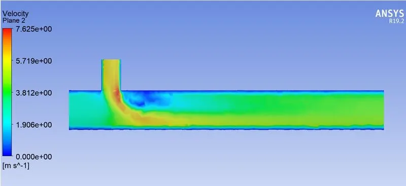
Temperature and velocity contour plots on the cut planes across the pipe
Velocity and temperature line plots along the length of the pipe.
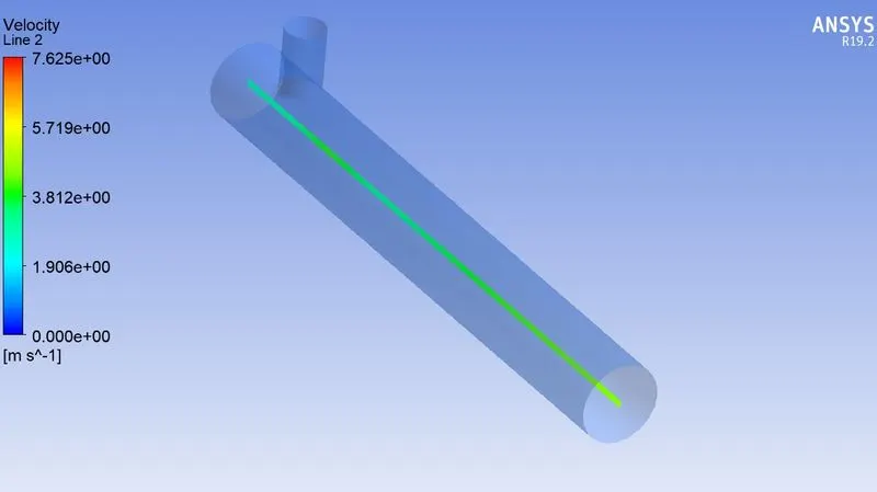
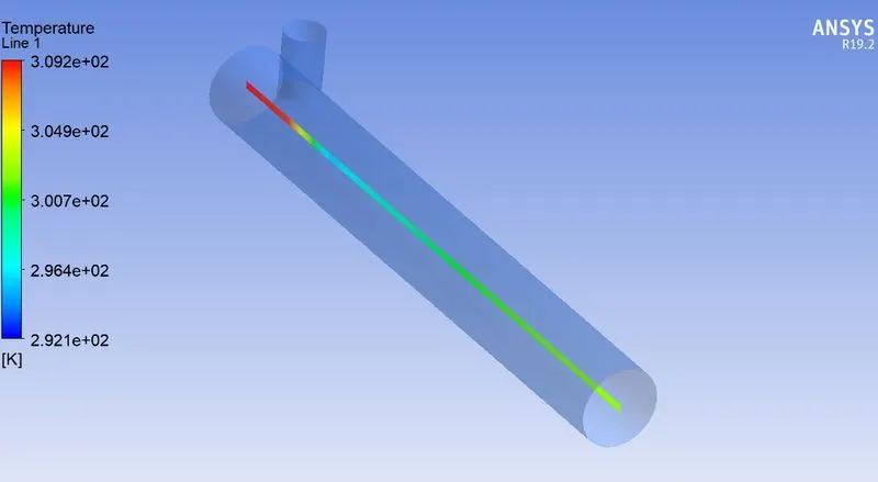
Velocity and temperature line plots across the length of the pipe.
5)Compairing Effectiveness of Mixing -
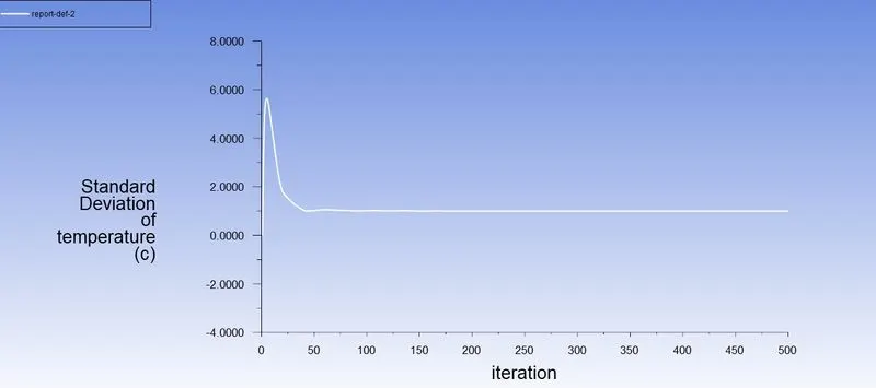
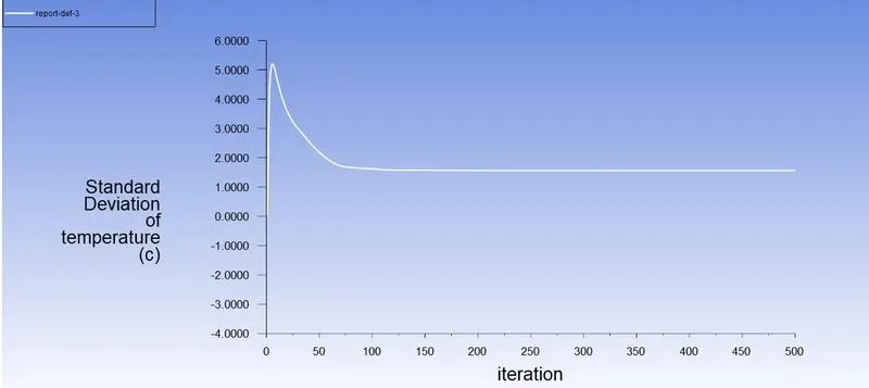
We can compare the mixing effectivenss by observing the plots of standard temperature deviation.A high standard deviation means the mixing is bad,while lower standard deviation means better mixing.Below is the comparison between standard devation of temperature for all the cases we have simulated.
Standard deviation of temperature for short T at Momentum Ratio 4 -
Standard deviation of temperature for short T at Momentum Ratio 2 -
Standard deviation of temperature for long T at Momentum Ratio 4 -
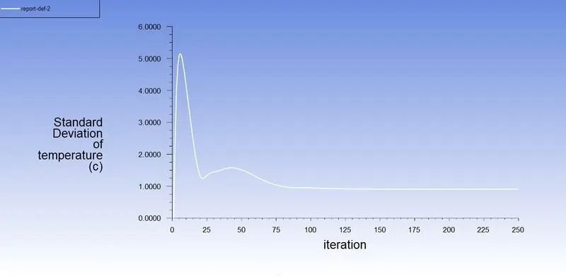
Standard deviation of temperature for long T at Momentum Ratio 2 -
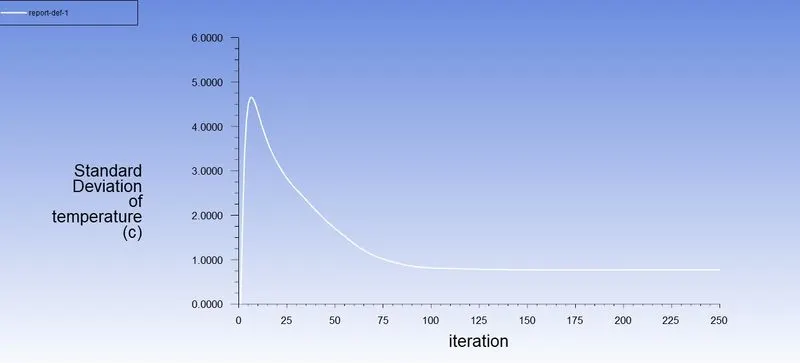
We can see that Tee's with higher momentum ratio has lower standard deviation compared to lower momentum ratio Tee's.Thus we are getting better mixing at high velocity flows and mixing effectivensss is loosely based on the length of the tee.This gets further validatedbby looking at contours of temperatue and velocity on the cut plane across the length of pipe.
6) Compairing Values from both cases -
| Long Tee. MR = 4 | Long Tee. MR = 2 | Short Tee. MR = 4 | Short Tee. MR =2 | |
| Cell Count | 15640 | 15640 | 12657 | 12657 |
| Average Outlet Temperature(C) | 27.481 | 30.320 | 27.487 | 30.223 |
| Average Outlet velocity(m/s) | 6.003 | 4.493 | 6.032 | 4.505 |
7)Mesh Independence -
It's a study to determine the dependence of the results on the mesh density.To do this,compare the results for various runs with
different mesh sizing.Thus we will run 2 simulation of different mesh sizing on short tee with momentum ratio 2 & 4.We will be sharing mesh and geometry file between two runs.
7.1)Output Results Table
At element size = 0.005
| Short Tee, MR=4 | Short Tee, MR=2 | |
| Cell Count | 14322 | 14322 |
| Average Outlet Temperature | 27.55 C | 30.211 C |
| Average Outlet Velocity | 6.027 | 4.504 |
At element size = 0.0025
| Short Tee, MR=4 | Short Tee, MR=2 | |
| Cell Count | 61985 | 61985 |
| Average Outlet Temperature | 27.579 C | 30.303 C |
| Average Outlet Velocity | 6.0180 | 4.495 |
Thus observing above table we can be sure that our case is grid independent.
8)Conclusion -
- As seen in high momentum ratio Tee's,mixing efficiency is better in them compared to low momentum ratio Tee's.
-Furthermore mixing efficiency less affected by the length of the pipe,though as the length of the pipe increases because of diffusion,flow always give slightely better mixing.
-k-epsilon predicts flow better away from the walls,while k-omega SST predicts better near the walls.
-At last,from all the given case we should use short tee with momentum ratio of 4,but we have to consider diffusion alog the length of the mixing tee,so long mixing tee with higher momentum ratio would be better option.