Week 7 - Simulation of a 1D Super-sonic nozzle flow simulation using Macormack Method
Objective :
To simulate the isentropic flow through a quasi 1D subsonic-supersonic nozzle,using the conservation and non-conservation forms of the governing equations and sovle them using the MacCormack's technique.
Description :
In this study,we are considering a convergent divergent nozzle shown in a below figure.The left side of the nozzle is connected to a reservoir.We assum thatcross-sectional area of the nozzle is very large(tends to infinity) and hence the inflow velocity is very small.The flow is locally subsonic(M<1) in convergent section,sonic at the throat(M=1) and supersonic(M>1) at the divergent section.The inlet pressure and temerature are given as `P_0` and `T_0`respectively .We assum, that the flow properties varies in x-direction only(area is a function of x),and hence it's a Quasi-1D-Flow.The flow is characterized as an isentropic,i.e. no heat added to the fluid and no energy transformations occur due to friction effects.
As area ratio is function of x,and mach number is the functionm of area ratio,it is in turn function of x.Also density ratio, pressure ratio and temperature ratio are function of mach number.To accelerate the flow at nozzle inlet some form of input is required,i.e pressure ratio.It supplies the required force to accelerate the flow through the nozzle inlet.For the given
area ratio,pressure ratio is fixed and is considered as a boundary condition.
In this study flow variables are considered in terms of non diamentional variables such as,`T' = T/T_0, P' = P/P_0, rho' = rho/rho_0,V' = V/a_0,x'=x/L`
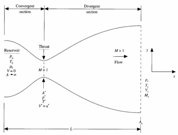
Fig. 1: Schematic for Subsonic-Supersonic Isentropic Nozzle Flow
Now let us consider a small control volume of the nozzle as shown below -
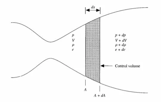
Fig2: Control Volume For Deriving PDE's
As mentioned above,we assum that,where the cross section area is A,the flow properties are uniform across the section. Hence,although the area of the nozzle changes as a function of distance along the nozzle,x,and therefore in reality the flow field is 2D(the flow varies in the 2D x-y space).We make the assumption that the flow properties vary only with x,this is tantamount to assuming uniform flow properties across any given cross-section.
The governing continuity,momentum and energy equations in terms of non dimentional variables for this Quasi-1D-Subsonic-Supersonic nozzle can be expressed as follows,
Non-Conservative Continuity Equation :
`(delrho')/(delt') = -rho'((delV')/(delx')) - rho'V'((del(ln A'))/(delx')) - V'((delrho')/(delx'))`
Non-Conservative Momentum Equation :
`(delV')/(delt') = -V'((delV')/(delx')) -(1/gamma)((delT')/(delx') + (T')/(rho')((delrho')/(delx'))`
Non-Conservative Energy Equation :
`(delT')/(delt') = -V'((delT')/(delx')) - (gamma -1)T'((delV')/(delx') + V'(del(lnA'))/(delx'))`
Conservative Continuity Equation :
`(del(rho'A'))/(delt') + (del(rho'A'V'))/(delx') = 0`
Conservative Momentum Equation :
`(del(rho'A'V'))/(delt') + (del[rho'A'(V')^2 +(1/gamma)rho'A'])/(delx') = (1/gamma)rho'((delA')/(delx'))`
Conservative Energy Equation :
`(del[rho'((e')/(gamma-1) + (gamma/2)(V')^2)A'])/(delt') + (del[rho'((e')/(gamma-1) + (gamma/2)(V')^2)V'A' + rho'A'V'])/(delx') = 0`
For air `gamma=1.4`
For the sake of calculation,let us simplify the conservative continuity,momentum and energy equations,
We are going to define solution vectors U,the flux vectors F,and the source term J as follows,
`U_1=rho'A'`
`U_2=rho'A'V'`
`U_3=rho'((e')/(gamma-1)+gamma/2V'^2)A'`
`F_1=rho'A'V'`
`F_2=rho'A'V'^2+1/gammap'A'`
`F_3=rho'((e')/(gamma-1)+gamma/2V'^2)V'A'+p'A'V'`
`J_2=1/gammap'(partialA')/(partialx')`
Using these elements the conservative continuity,momentum and energy equations can be written respectively as follows,
`(partialU_1)/(partialt')=-(partialF_1)/(partialx')`
`(partialU_2)/(partialt')=-(partialF_2)/(partialx')+J_2`
`(partialU_3)/(partialt')=-(partialF_3)/(partialx')`
Primitive variables are calculated as follows,
`rho'=U_1/(A'`
`V'=U_2/U_1`
`T'=e'=(gamma-1)((U_3)/(U_1)-gamma/2V'^2)`
`p'=rho'T'`
Initial conditions for conservative form are obtain from the Computational Fluid Dynamics by John D. Anderson,
`(( rho' =1.0),(T'=1.0))` for `0<=x'<=0.5`
`((rho'=1.0-0.366(x'-0.5)),(T'=1.0-0.167(x'-0.5)))` for `0.5<=x'<=1.5`
`((rho'=0.634-0.3879(x'-1.5)),(T'=0.833-0.3507(x'-1.5)))` for `1.5<=x'<=3.5`
`V'=(U_2)/(rho'A')=(0.59)/(rho'A'`
`A=1+2.2(x-1.5)^2`
Initial conditions for Non-conservative form at t=0,
`rho=1-0.3146x`
`T=1-0.2314x`
`V=(0.1+1.09x)T^(1/2)`
Boundary Conditions:
Non-Conservative Form-
Subsonic inflow boundary(point1)
`Vunderset1()=2Vunderset2()-Vunderset3`
Supersonic Outflow Boundary(point N)
`V_N=2V_(N-1)-V_(N-2)`
`rho_N=2rho_(N-1)-rho_(N-2)`
`T_N=2T_(N-1)-T_(N-2)`
Conservative Form-
Subsonic Inflow Boundary
`U_(1(i=1)=A'_(i=1)`
`U_(2(i=1))=2U_(2(i=2))-U_(2(i=3)`
`U_3=U_1((T')/(gamma-1)+gamma/2V'^2)`
Supersonic Outflow Boundary
`(U_1)_N=2(U_1)_(N-1)-(U_1)_(N-2)`
`(U_2)_N=2(U_2)_(N-1)-(U_2)_(N-2)`
`(U_3)_N=2(U_3)_(N-1)-(U_3)_(N-2)`
Mac-Cormack Method :
Mac-Cormack's technique is an explicit finite difference technique,that is second order accurate.It is a two step predictor-corrector sequence with forward difference for spatial derivatives in predictor step and backward difference for spatial derivatives in corrector step.The exact method is to first obtain the forward difference in predictor step for all the grid points in a perticular time step and then to otain the predicted values for all the primitive variables from the first two terms of a taylor series.Then the backward difference of the previously obtained predicted values is obtained in the corrector step.Once the predictor-corrector steps are obtaied,the average of the two steps is computed.In the end final solution is obtained from initial and average values.
1]Predictor step
`((partialrho)/(partialt))_i^t=-rho_i^(t)(V_(i+1)^t-V_(i)^t)/(Deltax)-rho_i^tV_(i)^t(lnA_(i+1)-lnA_(i))/(Deltax)-V_i^(t)(rho_(i+1)^t-rho_(i)^t)/(Deltax)`
2]Intermediate solution update
`rho_(i)^(t+Deltat)=rho_i^t+((partialrho)/(partialt))_i^tDeltat`
3]Corrector step
`((partialrho)/(partialt))_i^(t+Deltat)=-rho_i^(t+Deltat)(V_(i)^(t+Deltat)-V_(i-1)^(t+Deltat))/(Deltax)-rho_i^(t+Deltat)V_i^(t+Deltat)(lnA_(i)-lnA_(i-1))/(Deltax)-V_i^(t+Deltat)(rho_(i)^(t+Deltat)-rho_(i-1)^(t+Deltat))/(Deltax)`
4]Average time derivative
`((partialrho)/(partialt))_(ave)=0.5[((partialrho)/(partialt))_i^(t)+((partialrho)/(partialt))_(i)^(t+Deltat)]`
5]Final corrected values of the flow field variables at time `t+Deltat`
`rho_(i)^(t+Deltat)=rho_i^t+((partialrho)/(partialt))_(ave)Deltat`
Main Script :
clear all
close all
clc
%number of grid points
n = 31;
%length of nozzle
L=3;
%number of time steps
nt=1400;
%cfl number
C=0.5;
%specific heat ratio
gama=1.4;
%generating grid
x = linspace(0,L,n);
%grid spacing
dx=x(2)-x(1);
%area
A=1+2.2*(x-1.5).^2;
%calling conservative function
[rho_c,V_c,T_c,M_c,P_c,mfr_c,M_16,P_16,mfr_16,rho_16,T_16,V_16,t]=conservative(x,A,dx,n,nt,C,gama);
%calling non-conservative function
[rho_nc,V_nc,T_nc,M_nc,P_nc,mfr_nc,M_16_nc,P_16_nc,mfr_16_nc,rho_16_nc,T_16_nc,V_16_nc,t]=nonconservative(A,nt,C,n,gama,dx,x);

%Plotting Primitive Variable Distribution Inside The Nozzle
figure(1)
plot(x,rho_c)
hold on
plot(x,rho_nc,'*')
xlabel('length of nozzle')
ylabel('density')
legend('Conservative','Non-Conservative')
title('Density Distribution Inside The Nozzle')

figure(2)
plot(x,V_c)
hold on
plot(x,V_nc,'*')
xlabel('length of nozzle')
ylabel('velocity')
legend('Conservative','Non-Conservative')
title('Velocity Distribution Inside The Nozzle')

figure(3)
plot(x,T_c)
hold on
plot(x,T_nc,'*')
xlabel('length of nozzle')
ylabel('Temperature')
legend('Conservative','Non-Conservative')
title('Temperature Distribution Inside The Nozzle')


figure(4)
plot(x,P_c)
hold on
plot(x,P_nc,'*')
xlabel('length of nozzle')
ylabel('Pressure')
legend('Conservative','Non-Conservative')
title('Pressure Distribution Inside The Nozzle')

figure(5)
plot(x,M_c)
hold on
plot(x,M_nc,'*')
xlabel('length of nozzle')
ylabel('Mach Number')
legend('Conservative','Non-Conservative')
title('Mach Number Distribution Inside The Nozzle')

%Plotting Primitive Variable Distribution At The Throat
figure(6)
subplot(5,1,1)
plot([1:nt],rho_16)
hold on
plot([1:nt],rho_16_nc,'--k')
xlabel('Time step t')
ylabel('density')
title 'Time Wise Variation Of Density at Throat i=16'
legend('Conservative','Non-Conservative')

subplot(5,1,2)
plot([1:nt],T_16)
hold on
plot([1:nt],T_16_nc,'--k')
xlabel('Time step t')
ylabel('Temperatue')
title 'Time Wise Variation Of Temperature at Throat i=16'
legend('Conservative','Non-Conservative')


subplot(5,1,3)
plot([1:nt],V_16)
hold on
plot([1:nt],V_16_nc,'--k')
xlabel('Time step t')
ylabel('Velocity')
title 'Time Wise Variation Of Velocity at Throat i=16'
legend('Conservative','Non-Conservative')


subplot(5,1,4)
plot([1:nt],P_16)
hold on
plot([1:nt],P_16_nc,'--k')
xlabel('Time step t')
ylabel('Pressure')
title 'Time Wise Variation Of Pressure at Throat i=16'
legend('Conservative','Non-Conservative')

subplot(5,1,5)
plot([1:nt],M_16)
hold on
plot([1:nt],M_16_nc,'--k')
xlabel('Time step t')
ylabel('Mach Number')
title 'Time Wise Variation Of Mach number at Throat i=16'
legend('Conservative','Non-Conservative')

%Plotting Mass Flow Rate Variation Inside The Nozzle
figure(7)
plot(x,mfr_nc,'r')
hold on
plot(x,mfr_c,'b')
plot(x,0.579*ones(size(x)),'g')
xlabel('length of nozzle')
ylabel('Mass flow')
legend('Non-Conservative','Conservative','Analytical')
title('Mass Flow Variation')

%Plotting Time Wise Primitive Variable Variation Inside The Nozzle
figure(8)
subplot(5,1,1)
plot(linspace(1,nt,n),rho_c)
hold on
plot(linspace(1,nt,n),rho_nc,'--k')
xlabel('Time step t')
ylabel('density')
title 'Time Wise Variation Of Density'
legend('Conservative','Non-Conservative')

subplot(5,1,2)
plot(linspace(1,nt,n),T_c)
hold on
plot(linspace(1,nt,n),T_nc,'--k')
xlabel('Time step t')
ylabel('Temperatue')
title 'Time Wise Variation Of Temperature'
legend('Conservative','Non-Conservative')

subplot(5,1,3)
plot(linspace(1,nt,n),V_c)
hold on
plot(linspace(1,nt,n),V_nc,'--k')
xlabel('Time step t')
ylabel('Velocity')
title 'Time Wise Variation Of Velocity'
legend('Conservative','Non-Conservative')

subplot(5,1,4)
plot(linspace(1,nt,n),P_c)
hold on
plot(linspace(1,nt,n),P_nc,'--k')
xlabel('Time step t')
ylabel('Pressure')
title 'Time Wise Variation Of Pressure'
legend('Conservative','Non-Conservative')

subplot(5,1,5)
plot(linspace(1,nt,n),M_c)
hold on
plot(linspace(1,nt,n),M_nc,'--k')
xlabel('Time step t')
ylabel('Mach Number')
title 'Time Wise Variation Of Mach Number'
legend('Conservative','Non-Conservative')


figure(9)
plot(linspace(1,nt,n),mfr_nc,'r')
hold on
plot(linspace(1,nt,n),mfr_c,'b')
xlabel('length of nozzle')
ylabel('Mass flow')
legend('Non-Conservative','Conservative')
title('Time Wise Mass Flow Variation')
Function for Conservative Form :
function [rho,V,T,M,P,mfr,M_16,P_16,mfr_16,rho_16,T_16,V_16,t]=conservative(x,A,dx,n,nt,C,gama)
%initial conditions
for k=1:n
    if x(k)>=0 && x(k)<=0.5
        rho(k)=1;
        T(k)=1;
    elseif x(k)>0.5 && x(k)<=1.5
        rho(k)=1-0.366*(x(k)-0.5);
        T(k)=1-0.167*(x(k)-0.5);
    elseif x(k)>1.5 && x(k)<=3.5
        rho(k) = 0.634-0.3879*(x(k)-1.5);
        T(k)=0.833-0.3507*(x(k)-1.5);
    end
end

        V=0.59./(rho.*A);
        U1=rho.*A;
        U2=U1.*V;
        U3=U1.*((T/(gama-1))+(gama/2).*V.^2);

 %timestep calculation
        for i=1:n
        u=(T(i))^(1/2);
        t_step(i)=C*dx/(u+V(i));

  end
       dt=min(t_step);

%time loop
for t=1:nt

   %keeping copy of initial values
        U1_initial=U1;
        U2_initial=U2;
        U3_initial=U3;

        F1_p=U2;
        F2_p=(U2.^2./U1)+((gama-1)/gama)*(U3-(gama/2)*(U2.^2./U1));
        F3_p=(gama*(U2.*U3)./U1)-((gama*(gama-1)/2)*U2.^3./U1.^2);

    %MacCormack method

    %predictor loop

    for i=2:n-1

    %predictor time derivatives calculation
        dU1dt_p(i)= -(F1_p(i+1)-F1_p(i))/dx;
        J2_p(i)=(1/gama)*rho(i).*T(i).*(A(i+1)-A(i))/dx;%source term
        dU2dt_p(i)=-((F2_p(i+1)-F2_p(i))/dx)+J2_p(i);
        dU3dt_p(i)=-(F3_p(i+1)-F3_p(i))/dx;

    %intermediate values
        U1(i)=U1_initial(i)+dU1dt_p(i)*dt;
        U2(i)=U2_initial(i)+dU2dt_p(i)*dt;
        U3(i)=U3_initial(i)+dU3dt_p(i)*dt;
    end
    %calculating primitive variables
        rho=U1./A;
        T=(gama-1)*(U3./U1-(gama/2)*(U2./U1).^2);
        V=U2./U1;
        P=rho.*T;
        M=V./T.^(1/2);
        mfr=rho.*A.*V;
    %updating flux terms
        F1_c=U2;
        F2_c=(U2.^2./U1)+((gama-1)/gama)*(U3-(gama/2)*(U2.^2./U1));
        F3_c=(gama*U2.*U3./U1)-((gama*(gama-1)/2)*U2.^3./U1.^2);


    %corrector loop
    for i=2:n-1
    %corrector time derivatives calculation
        dU1dt_c(i)= -(F1_c(i)-F1_c(i-1))/dx;
        J2_c(i)=(1/gama)*rho(i).*T(i).*(A(i)-A(i-1))/dx;%source term
        dU2dt_c(i)=-((F2_c(i)-F2_c(i-1))/dx)+J2_c(i);
        dU3dt_c(i)=-(F3_c(i)-F3_c(i-1))/dx;


    %calculating average time derivative
        dU1dt_avg(i)=0.5*(dU1dt_c(i)+dU1dt_p(i));
        dU2dt_avg(i)=0.5*(dU2dt_c(i)+dU2dt_p(i));
        dU3dt_avg(i)=0.5*(dU3dt_c(i)+dU3dt_p(i));

    %update solution vector
        U1(i)=U1_initial(i)+dU1dt_avg(i)*dt;
        U2(i)=U2_initial(i)+dU2dt_avg(i)*dt;
        U3(i)=U3_initial(i)+dU3dt_avg(i)*dt;
    end

    %inlet boundary conditions
        U1(1)=A(1);
        U2(1)=2*U2(2)-U2(3);
        U3(1)= U1(1)*((T(1)/(gama-1))+((gama/2)*(U2(1)/U1(1))^2));

    %outlet boundary conditions
        U1(n)=2*U1(n-1)-U1(n-2);
        U2(n)=2*U2(n-1)-U2(n-2);
        U3(n)=2*U3(n-1)-U3(n-2);

    %calculating primitive variables
        rho=U1./A;
        V=U2./U1;
        T=(gama-1)*((U3./U1)-(gama/2)*V.^2);
        M=V./T.^(1/2);
        P=rho.*T;
        mfr=rho.*A.*V;
   %primitive variables at throat(i=16)(a=1)
        rho_16(t)=rho(16);
        T_16(t)=T(16);
        V_16(t)=V(16);
        M_16(t)=M(16);
        P_16(t)=P(16);
        mfr_16(t)=mfr(16);

   %Plotting Variation Of Mass Flow Rate Inside Nozzle At Different Time Steps

        figure(10)
if t==1
    plot(x,mfr,'color','b')
    hold on
elseif t==50
    plot(x,mfr,'color','r')
    hold on
elseif t==100
    plot(x,mfr,'color','g')
    hold on
    elseif t==400
    plot(x,mfr,'color','k')
    hold on
    elseif t==700
    plot(x,mfr,'color','c')
    hold on
    elseif t==1000
    plot(x,mfr,'color','m')
    hold on
    elseif t==1400
    plot(x,mfr,'color','y')
    hold on
end
hold on
xlabel('Nozzle Length')
ylabel('Mass Flow Rate')
title 'Conservative Mass Flow Rate At Different Time Steps'
end %end of time loop
legend ('nt=1','nt=50','nt=100','nt=400','nt=700','nt=1000','nt=1400')
end %end of function
Function for Non-Conservative Form :
function [rho,V,T,M,P,mfr,M_16,P_16,mfr_16,rho_16,T_16,V_16,t]= nonconservative(A,nt,C,n,gama,dx,x)
 %initial conditions at t=0
        rho=1-0.3146*x;
        T=1-0.2314*x;
        V=(0.1+(1.09*x)).*T.^(1/2);

 %time loop
   for t=1:nt

   %timestep calculation
   for i=1:n
        u=(T(i))^(1/2);
        t_step(i)=C*dx/(u+V(i));
   end
        dt=min(t_step);

    %keeping copy of initial values
        rho_initial=rho;
        V_initial=V;
        T_initial=T;

     %McCormack method

  for i=2:n-1
     %predictor step
        drhodx=(rho(i+1)-rho(i))/dx;
        dVdx=(V(i+1)-V(i))/dx;
        dlnAdx=(log(A(i+1))-log(A(i)))/dx;
        dTdx=(T(i+1)-T(i))/dx;
     %calculating predictor time derivative
        drhodt_p=-rho(i)*dVdx-rho(i)*V(i)*dlnAdx-V(i)*drhodx;
        dVdt_p=-V(i)*dVdx-(1/gama)*(dTdx+(T(i)/rho(i))*drhodx);
        dTdt_p=-V(i)*dTdx-(gama-1)*T(i)*(dVdx+V(i)*dlnAdx);

     %solution update
        rho(i)=rho(i)+drhodt_p*dt;
        V(i)=V(i)+dVdt_p*dt;
        T(i)=T(i)+dTdt_p*dt;

     %corrector step

        drhodx_c=(rho(i)-rho(i-1))/dx;
        dVdx_c=(V(i)-V(i-1))/dx;
        dlnAdx_c=(log(A(i))-log(A(i-1)))/dx;
        dTdx_c=(T(i)-T(i-1))/dx;

     %corrector time derivatives calculation

        drhodt_c=-rho(i)*dVdx_c-rho(i)*V(i)*dlnAdx_c-V(i)*drhodx_c;
        dVdt_c=-V(i)*dVdx_c-(1/gama)*(dTdx_c+(T(i)/rho(i))*drhodx_c);
        dTdt_c=-V(i)*dTdx_c-(gama-1)*T(i)*(dVdx_c+V(i)*dlnAdx_c);

     %calculating average time derivative
        drhodt_avg=0.5*(drhodt_c+drhodt_p);
        dVdt_avg=0.5*(dVdt_c+dVdt_p);
        dTdt_avg=0.5*(dTdt_c+dTdt_p);

     %final solution update
        rho(i)=rho_initial(i)+drhodt_avg*dt;
        V(i)=V_initial(i)+dVdt_avg*dt;
        T(i)=T_initial(i)+dTdt_avg*dt;
  end
     %outlet boundary conditions
        V(n)=2*V(n-1)-V(n-2);
        rho(n)= 2*rho(n-1)-rho(n-2);
        T(n)= 2*T(n-1)-T(n-2);
      %inlet boundary condition
        rho(1)=1;
        T(1)=1;
        V(1)=2*V(2)-V(3);

        M=V./T.^(1/2);
        P=rho.*T;
        mfr=rho.*A.*V;
     %primitive variables at throat
        rho_16(t)=rho(16);
        T_16(t)=T(16);
        V_16(t)=V(16);
        P_16(t)=P(16);
        M_16(t)=M(16);
        mfr_16(t)=mfr(16);


     %Plotting Variation Of Mass Flow Rate Inside Nozzle At Different Time Steps
         figure(11)
if t==1
    plot(x,mfr,'color','b')
    hold on
elseif t==50
    plot(x,mfr,'color','r')
    hold on
elseif t==100
    plot(x,mfr,'color','g')
    hold on
    elseif t==400
    plot(x,mfr,'color','k')
    hold on
    elseif t==700
    plot(x,mfr,'color','c')
    hold on
    elseif t==1000
    plot(x,mfr,'color','m')
    hold on
    elseif t==1400
    plot(x,mfr,'color','y')
    hold on
end
hold on
xlabel('Nozzle Length')
ylabel('Mass Flow Rate')
title 'Non Conservative Mass Flow Rate At Different Time Steps'
        end        %end of time loop
legend ('nt=1','nt=50','nt=100','nt=400','nt=700','nt=1000','nt=1400')
end                %end of function
Plots and Discussing Results :
Variation of Properties Along the Nozzle: Conservative Vs Non-Conservative
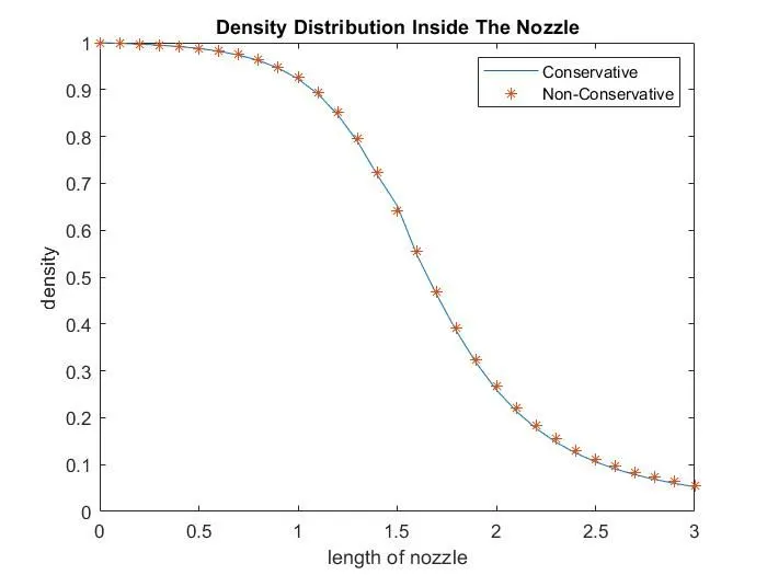
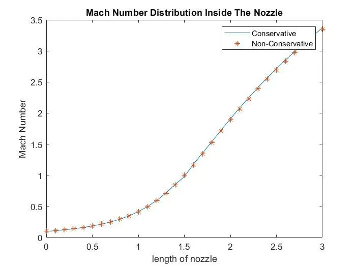
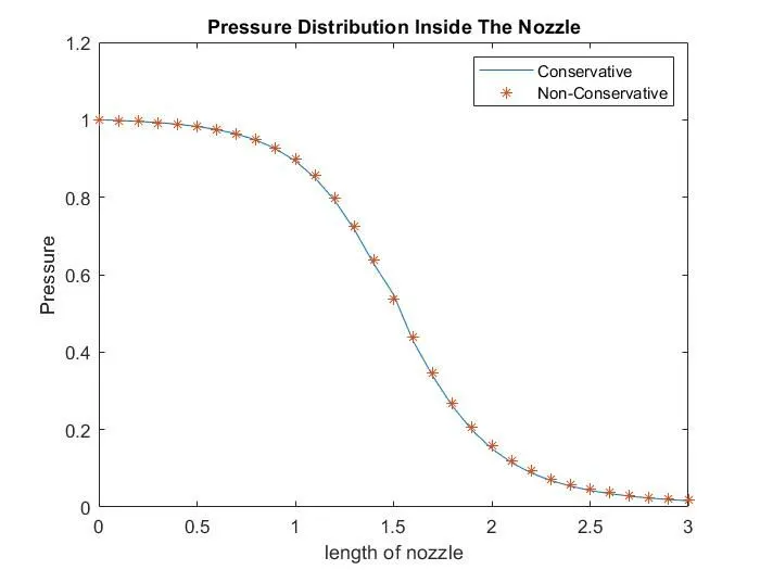
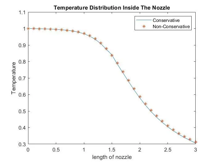
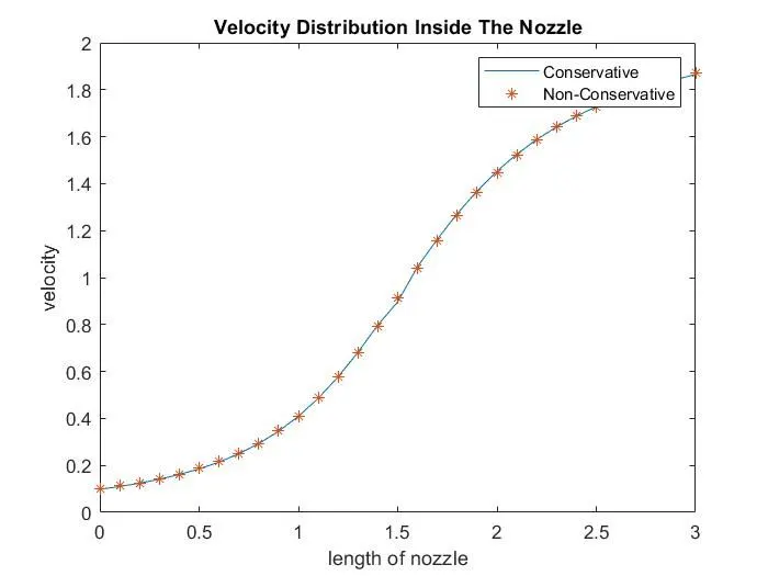
The above plots shows the variation of diffferent flow properties along the length of the nozzle.
We can see that temperature,density & pressure decreases,while velocity and Mach number increases,which is logical as the flow moves from convergent section to divergent section.
Time Wise Variation Of Properties At Throat : Conservative Vs Non-Conservative
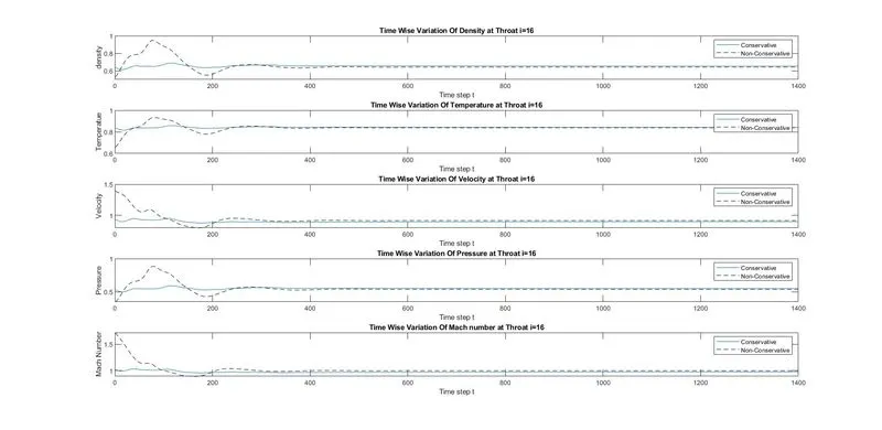
From the above plots ,we can see that at lower time steps,the properties oscillate,but after certain number of time steps i.e. around 400 ,the solution converges.Also we can see ,that in consevative form it takes lower number of timesteps to converge compare to non-conservative form.Also,there are less oscillations in consevative form compared to non conservative form.
Mass Flow Variation At Different Time Steps :-
Conservative Form :
Non-Conservative Form :
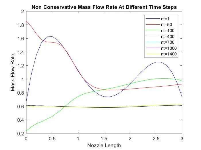
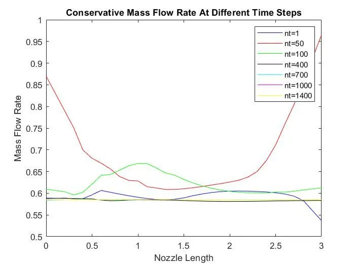
After Observing the above plots we can conclude that normally it takes minimum 700 time steps are required for convergence because,after that results are same as we can see for 1000 & 1400 time steps.
Steady State Mass Flow Variation :
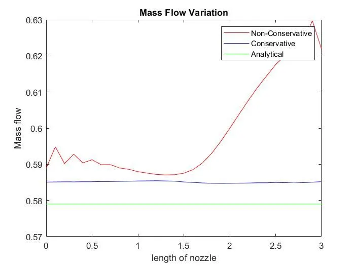
We can see that steady state mass flow is less significant in the case of conservative form as the flux variable `U_2=rho*V*A` is used to compute the solution.And since non-conservative form uses primitive variables `rho,V,T` hence the variation is signiicant.
Therefore we can conclude that steady state mass flow distibution predicted by conservative form is satisfactory compared to non-conservative form.
Grid Independence Test :-
Lets consider flow at the throat section.The comparison of different flow variables at the throat shows,that the results do not vary significantly,with increase in grid points.In other words we can say, that the solution obtained at 31 grid points is a grid independent solution.
| Number of Grid Points | Pressure | Density | Temperature | Mach Number |
| 31(Conservative) | 0.548 | 0.652 | 0.841 | 0.978 |
| 31(Non-Conservative) | 0.538 | 0.642 | 0.838 | 0.999 |
| 61(Conservative) | 0.534 | 0.639 | 0.835 | 0.997 |
| 61(Non-Conservative) | 0.535 | 0.639 | 0.836 | 0.999 |