Week 8: Literature review - RANS derivation and analysis

Aim :

To apply Reynold's decomposition to the NS equations and come up with the expression for Reynold's stress.
Also understanding of the terms reynold's stress and turbulent viscosity.And How turbulent viscosity is different from molecular viscosity.

Objective :

The objective of this literature review is to apply the REynolds decomposition process to NS equations and derive an expression for Reynolds stress and also to understand the difference between the turbulent viscosity and molecular viscosity.

Intoduction And Theory :

RANS is a numerical method to model a turbulent flow wherein the flow quantities are decomposed into their time-averaged and fluctuating components (Reynolds decomposition).The averaging of Navier-Stokes equations yields a nonlinear Reynolds stress term that requires additional modeling to fully resolve the system(Turbulence model).Most (if not all) RANS turbulence models are based on empirical observations.

The Navier-Stokes equations are arguably among the most complex to use and solve in mathematical physics. This set of coupled time-dependent nonlinear equations requires many approximations in order to reach analytical solutions, and not all systems are solvable. For more general systems or complex geometries, numerical techniques are needed to solve these equations and derive useful insights into flow behavior. Some mathematical approximations can be used to reduce the complexity of these equations, which will help speed up simulations without losing too much accuracy.

The Reynolds-averaged Navier-Stokes (RANS) equations are a reduced form of the general Navier-Stokes equations. In the RANS equations, the steady-state solution is decoupled from the time-varying fluctuations in the system, the latter of which will account for turbulence in different flow regimes.

An Overview of the Reynolds-Averaged Navier-Stokes (RANS) Equations :

The technique used to derive the RANS equations is called Reynolds decomposition. Reynolds averaging and Reynolds decomposition do not refer directly to a manipulation of the Reynolds number, but rather to an application of time averaging to the Navier-Stokes equations. Time averaging is often used to reduce complex systems of differential equations into simpler forms by partially or fully eliminating the time variable. In this case, the RANS equations use a solution that is split into a time-independent mean flow velocity and time-varying fluctuations.

Turbulence Analysis :

Let's take a look at instantaneous velocity measurements in turbulent flows.

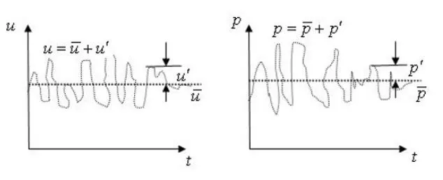
Fig. : Fluctuating And Mean Velocity And Pressure

Fluctuations can be of small scale and high frequency.They are computationally too expensive to simulate directly in practical engineering applications.
Instead,the instantaneous governing equations can be time averaged,ensemble-averaged or otherwise manipulated to remove the small scales,resulting in a
modified set of equations that are computationally less expensive to solve.However,modified equations contains additional unknown variables,and turbulence models
are needed to determine these variables in terms of known quantities.

Turbulence Modelling :

Turbulence modelling is used to calculate Reynold's stress and turbulent viscosity.The effect of turbulence can be modelled using a method called as Direct Numerical Simulation(DNS),which involves solving Navier Stokes equation over turbulent time step.But the turbulent time step is very small thus computational cell size is required to solve.Thus,turbulence model is used to capture the effect of turbulence in coarse grid size.

Different turbulence models are as follows -
*Reynolds Average Navier Stokes Equation(RANS)
*Large Eddy Simulation (LES)
*Direct Numerical Simulation(DNS)

Navier-Stokes Equations :
The NS equations govern the motion of fluids and can be seen as Newton's second law of motion for fluids.The equations consists of solving the continuity equation,momentum equation and energy equation of a fluid together.

Continity Equation :

`(delu)/(delx)+(delv)/(dely)= 0`

Momentum Equation :

`rho{(delu)/(delt)+u*(delu)/(delx)+v*(delu)/(dely)}=-(delP)/(delx)+mu*(del^2u)/(dely^2)`

Energy Equation :

`rho_c{(delT)/(delt)+u*(delT)/(delx)+v*(delT)/(dely)}=k(del^2T)/(delx^2)+mu*((delu)/(dely))^2`

Reynolds Average Navier Stokes Equation(RANS) :

Two alternative methods can be employed to transform navier stokes equations in such a way that the small scale turbulent fluctuations do not have to be directly simulated,those are reynolds averaging and filtering.Both methods introduces additional terms into the governing equation that needs to be modelled in order to achive closure.(Closure implies that there are a sufficient number of equations for all the unknowns.)

The rationale for Reynold's averaging is that we are not interested in the part of the flow solution that can be described as 'turbulent fluctuations' instead,it is the mean (velocity,pressure,lift,drag)that is of interest. RANS equations represent transport equations for the mean flow quantities only,with all the scales of the turbulence being modelled.The approach of permitting a solution for the mean flow variables greatly reduces the computational effort.

Reynolds Decomposition :

The RANS equations are time averaged equations of motion for fluid flow.The idea behind the equation is Reynold's decomposition whereby an instantaneous quantity is decomposed into it's time averaged and fluctuating quantities.For example,
u(x,y,z,t)=baru(bar(x,y,z,t))+u'(x,y,z,t)
where,momentary velocity component is u(x,y,z,t),the time averaged value is baru(bar(x,y,z,t)) and the fluctuating velocity is u'(x,y,z,t).

To apply the Reynolds decomposition to the NS equation,we need to substitute the Reynold's decomposition method by introducing time averaged values and fluctuating values into the basic NS equation.

Reynold's Decomposition,

Instantaneous Velocity(At any point in space and time) =Time Averaged Quantity +Fluctuating Component

Time averaged velocity for steady flow, u_t(x)=1/Tint_0^Tu(x,t)dt

Time averaged velocity for unsteady flow, u_t(x,t_n)=1/Tint_(t_n-1/2)^(t_n+1/2T)u(x,t)dt

For unsteady flow the T is the spontaneous time period which is shorter than the entire time period,therefore the entire velocity is time dependent. Reynolds decomposition used for the derivation is as follows,
u = U + u'
p = P + p'

in 3D flow,
u(x,y,z,t)=u(x,y,z) + u'(x,y,z,t) -----eq.A
v(x,y,z,t)=v(x,y,z) + v'(x,y,z,t)
w(x,y,z,t)=w(x,y,z) + w'(x,y,z,t)

Time Averaged Quantities :

baru(x,y)=1/t_iint_0^(t_i)u(x,y,z,t)dt

Since we are integrating,we get average quatites and these average quantities does not change with time,Therefore `baru` is f(x,y). Thus eq.A implies that,

`1/t_iint_0^(t_i)u(x,y,z,t)dt=1/t_iint_0^(t_i)baru(x,y,z)dt+1/t_iint_0^(t_i)u'(x,y,z,t)dt`

Where,`baru` is not a function of time.

Hence when we integrate the fluctuationg component,it will always be zero.

1/t_iint_0^(t_i)u'(x,y,z,t)dt=0

Therefore,when we integrate the fluctuating terms for longer time period this term would be ZERO.

Continuity Equation :

`(delu)/(delx)+(delv)/(dely)= 0`

Applying Reynolds Decomposition,

`1/t_iint_0^(t_i)del/(delx)(baru+u')dt+1/t_iint_0^(t_i)del/(dely)(barv+v')dt=0`

`1/t_iint_0^(t_i)del/(delx)barudt+1/t_iint_0^(t_i)del/(delx)u'dt+1/t_iint_0^(t_i)del/(dely)barvdt+1/t_iint_0^(t_i)del/(dely)v'dt=0`

Time integration of fluctuating component is zero and also integral limit is not a function of x.

`1/t_iint_0^(t_i)del/(delx)barudt+1/t_iint_0^(t_i)del/(dely)barvdt=0`

`del/(delx)baru*(1/t_i)int_0^(t_i)dt+del/(dely)barv*(1/t_i)int_0^(t_i)dt=0`

`del/(delx)baru((t_i-0)/t_i)+del/(dely)barv((t_i-0)/(t_i))=0`

`del/(delx)baru+del/(dely)barv=0`

Thus Reynold's decomposition satisfies continuity equation.

Momentum Equation :

`rho{(delu)/(delt)+u*(delu)/(delx)+v*(delu)/(dely)}=-(delP)/(delx)+mu*(del^2u)/(dely^2)`

Moving density to R.H.S.

`(delu)/(delt)+u*(delu)/(delx)+v*(delu)/(dely)=-1/rho(delp)/(delx)+(mu/rho)*((del^2u)/(dely^2))`

Replacing `mu/rho=nu`

where `nu`=kinematic viscosity

`(delu)/(delt)+u*(delu)/(delx)+v*(delu)/(dely)=-1/rho(delp)/(delx)+nu*((del^2u)/(dely^2))`

Now we will add x component of velocity multiplied by continuity equation,

`(delu)/(delt)+u*(delu)/(delx)+v*(delu)/(dely)+u((delu)/(delx)+(delv)/(dely))=-1/rho(delP)/(delx)+nu(del^2u)/(dely^2`

Adding continuity equation doesn't disbalance the equaton,as it has already been proved that it is equal to zero.

Combining both x-component equations,

`(delu)/(delt)+2u*(delu)/(delx)+v*(delu)/(dely)+u*(delv)/(dely)=-(1/rho)(delP)/(delx)+nu*(del^2u)/(dely^2)`

Lets further simplify using the Product Rule

`(del(u.v))/(dely) = u*(delv)/(dely)+v*(delu)/(dely)`

Therefore,

`(delu)/(delt)+2u*(delu)/(delx)+(del(u*v))/(dely)=-(1/rho)(delP)/(delx)+nu*(del^2u)/(dely^2)`

Integrating w.r.t. time(`t_i`) and applying Reynolds decomposition

`1/t_i*int_0^(t_i){(del/(delt)(baru+u')dt)+del/(dely)(baru+u')(barv+v')dt+del/(delx)(baru+u')^2dt}=1/(t_i)int_0^(t_i){[-del/(rhodelx)(barP+P')dt]+nudel^2/(dely^2)(baru+u')dt}`

Splitting into multiple integrals

`1/(t_i)int_0^(t_i){(delbaru)/(delt)dt+(delu')/(delt)dt+(delbaru^2)/(delx)dt+(delu'^2)/(delx)dt+(del((2*baru*u')/(delx))dt+(del)/(dely)(barubarv)dt+(del)/(dely)(baruv')dt+(del)/(dely)(u'barv)dt+(del)/(dely)(u'v')dt=1/(t_i)int_0^(t_i){-1/(rho)*(delbarP)/(delx)dt-(1/rho)*(delP')/(delx)dt+nu(del^2baru)/(dely^2)dt+nu(del^2u')/(dely^2)dt}`

Time average of fluctuating components is zero.

`(delbaru)/(delt)+(delbaru^2)/(delx)+(del)/(dely)(baru*barv)=-(1/rho)*(delbarP)/(delx)+nu*(del^2baru)/(dely^2)-(1/t_i)int_0^(t_i)(del)/(delx)(u')^2dt-(1/t_i)int_0^(t_i)(del)/(dely)(u'v')dt`

Now if we consider that the u' value is fluctuating between -1 and 1 then by averaging it,the value of u' comes to 0,but if we consider the same case for `(u')^2` then during averaging the square of -1 becomes 1 and the averaged value comes out to be a positive value and not zero which when integrated will never give a zero value and thats why ,technically the term `1/t_iint_0^(t_i)(del(u')^2)/(delx)dt` is not equal to zero.

Simillarly,in the term `t/t_iint_0^(t_i)(del(u'*v'))/(dely)dt`,the fluctuations along x axis(u') and the fluctuations along the y axis (v') are co related.That is,when a low momentum y component is flowing in the +ve y-direction then the high momentum(i.e.high velocity) x-component gets slowed down which is caused by v'.So the +ve increase in v' is going to cause a -ve result in u' and the product of the two (u'.v') will come out to be a -ve value only.Hence the integration of the -ve value will result into a -ve value which means that this term won't be 0 as well.

In order to simplify this equaion furthermore an assumption is required to be made.The term `int_0^(t_i)(del(u')^2)/(delx)dt` is in a boundary layer,and boundary layers are very thin in comparison to the plate and in that small space the velocity gradient in y-direction changes a lot,though the change in the velocity in x-direction is very less when compared to that in y-direction and hence this term can be neglected.This is only true in the case of a boundary layer.

Further simplification

`(delbaru)/(delt)+(delbaru^2)/(delx)+(delbarubarv)/(dely)=-1/(rho)(delbarP)/(delx)+nu*(del^2baru)/(dely^2)-(1/t_i)int_0^(t_i)(del(u'v'))/(dely)dt`

Take out `1/rho*del/(dely` from R.H.S.

`(delbaru)/(delt)+(delbaru^2)/(delx)+(delbarubarv)/(dely)=-(1/rho)*(delbarP)/(delx)+(1/rho)(del)/(dely){nu*(delbaru)/(dely)-rho/t_iint_0^(t_i)[(u'v')dt]}`

Where,

`(delbaru)/(delt)+(delbaru^2)/(delx)+(delbarubarv)/(dely)` = Inertial Term

`-(1/rho)*(delbarP)/(delx)` = Pressure Term

`nu*(delbaru)/(dely)`= Molecular Visocity or Viscous Stress

`rho/t_iint_0^(t_i)[(u'v')dt]` = Momentum diffusivity due to turbulence or Reynold's stress.

Reynolds Stress :

In fluid dynamics,the reynolds stress is the component of total stress tensor in a fluid ,obtained from the averaging operation over the NS equations to account for turbulent fluctuations in fluid momentum.

This stress offers significant effects for the complex interactions in turbulent flows.This stress can be used to model the Reynolds stress transport equation which will allow using the comparatively larger grid to flow analysis.

What is turbulent viscosity?How is it different from molecular viscosity ?

Turbulent viscosity is the coefficient that relates the average shear stress and the rate of velocity gradient in the turbulent flow.The viscosity in turbulent flow is non homogenous and it varies in space.

The turbulent transfer of momentum by eddies giving rise to an internal fluid friction ,in a manner analogous to the action of molecular viscosity in laminar flow,but taking place on a much larger scale.It is greater for flows eith more turbulence .

In,a turbulent fluid,a linear interface between two different fluids breaks apart to form small scale structures also known as eddies.As these eddies grow and diminsh in size(by energy cascades),they effectively alter the surface area of interface between the fluids with different properties,thus altering the net transfer of momentum and the scalar properrties through the interfaces.

In the CFD simulations the size of the girid boxes determines the smallest scale of the eddies that the machine can resolve .In other words if the grid size of th edomain is huge ,then net effective momentum transfers due to small eddies occuring within the box os unknown to the machine.In order to estimate net effective mixing at each of these grid boxes,we specify an effective viscosity and multiply it with the shear(or velocity gradient) of the fluid surrounding th egrid box.This effective viscosity is called turbulent viscosity.The product of turbulent viscosity and shear gives us the net diffusive flux of fluid across the grid box.For momentum that would be diffusive momentum flux and for density/temperature that would be scalar flux.

Molecular Viscosity :

Molecular Viscosity = `tau_(i,j)=mu(du_i)/(dy_j)`

Molecular viscosity is same as viscosity.The coefficient of molecular viscosity is the same value as dynamic viscosity(`mu`).Molecular viscosity is the transport of mass motion momentum solely by the random motions of individual molecules not moving together in coherent groups.Molecular viscosity is analogous in laminar flow to eddy viscosity in turbulent flow.It can be considered as some sort of internal friction between two layers of the fluid developed while flowing.

Difference Between Molecular Viscosity and Turbulent Viscosity :

• Turbulent viscosity is an imaginary concept but molecular viscosity is a dynamic viscosity that will be present in all real fluids.
• Molecular viscosity depends only on the properties of the fluid,while turbulent viscosity depends on the properties of fluid flow like velocity,pressure,reynolds number etc.
• Molecular viscosity is present in all types of flows,but turbulent viscosity is present only in turbulent flows.
• Molecular viscosity is dominant in low Re flows (i.e.laminar region),and turbulent viscosity is dominant in high Re flows(i.e.turbulent regions)
• Molecular Viscosity is linear ans easy to measure ,whereas turbulent viscosity is non linear and difficult to measure.

Conslusion :

Hence we have successfully derived the expression for Reynolds stress by applying the Reynold's decomposition to the Navier-Stokes equations.We have also described what is Reynolds stress as well as turbulent viscosity,and showed the difference between molecular viscosity and turbulent viscosity.