Week 5.1 - Mid term project - Solving the steady and unsteady 2D heat conduction problem

Objective -

To Solve the 2D heat conduction equation by using the point iterative techniques.

Problem Statement-

Solve the 2D heat conduction equation by using the point iterative techniques.

1) The Boundary conditions for the problem are as follows -

Top Boundary = 600 K

Bottom Boundary = 900 K

Left Boundary = 400 K

Right Boundary = 800 K

2) Absolute error criteria 1e-4.

3)the following methods will be implimented for solving implicit equations.

A. Jacobi

B. Gauss-seidel

C. Successive over-relaxation

4)Assum nx=ny=10.

5)All the nodes except boundary nodes will be at initial temperature = 300k.

6)We will solve the steady state 2D heat conduction by Jacobi Method,Gauss Seidel Method & Successive over
relaxation(SOR) method and transient/unsteady state by explicit and prior mentioned iterative methods.

Explaination-

We know the 2D heat conduction equation,.

`(delT)/(delt) = alpha((del^2T)/(delx^2))+((del^2T)/(dely^2))`

where,

T =temperature

t=time

alpha = thermal expansion coefficient

Steady State 2D Heat Conduction Equation -

`((del^2T)/(delx^2))+((del^2T)/(dely^2)) = 0`

After using central defference discretization ,the above equation

`T_(i,j)^n = 1/k*[(T_(i+1,j)^n + T_(i-1,j)^n)/(Deltax^2) + (T_(i,j+1)^n + T_(i,j-1)^n)/(Deltay^2)]`

where,

`k = 2*((Deltax^2+Deltay^2)/(Deltax^2*Deltay^2))`

Transient 2D heat conduction equation-

For Explicit Scheme-

`(delT)/(delt) + alpha((del^2T)/(delx^2)+(del^2T)/(dely^2)) = 0`

hence we get,

`T_P^(n+1) = T_P^n(1-2k_1-2k_2) + k_1T_L^n+ k_1T_R^n + k_2T_B^n + k_2T_T^n`

where,
k_1 =( alpha*Deltat)/(Deltax^2)
&
k_2 = ( alpha*Deltat)/(Deltay^2).

For Implicit Scheme-

`T_P^(n+1)*(1+2k_1 + 2k_2) = T_P^n + k_1(T_L^(n+1)+ T_R^(n+1)) + k_2(T_T^(n+1) + T_B^(n+1))`

Code Explaination-

After defining all the inputs,I initialize a 10 * 10 matrix T ,and gave top,bottom,left & right boundaty temperatures.
Then define dummy variable and tolerance value for convergence.I created function for each iterative solver and called
them into the main program.Then plotted the temperature distribution,to do this I used contourf to create filled contour plot.
To indicate the mapping of temperature values I used colorbar.In the function of each method after running space loop,I updated temperature values so that the latest temperature value gets use in next iteration.Also updated the initial temperature values to get use in next time step.

Matlab Code-

For Steady State

Main code

%Solving 2D Steady state and transient heat conduction equation
clear all
close all 
clc
%Inputs
nx = 20;
ny = nx;
x = linspace(0,1,nx);
y = linspace(0,1,ny);
dx =x(2)-x(1);
dy = y(2)-y(1);
T = 300*ones(nx);
T(:,1) = 400;
T(:,nx) = 800;
T(1,:) = 600;
T(ny,:) = 900;
k = 2*(dx^2+dy^2)/(dx^2*dy^2);
tolerance = 1e-4; %Absolute error criteria
Told=T;

% JACOBI FOR STEADY STATE
[T,j_iter]= jacobi(nx,ny,k,dx,dy,Told,T,tolerance);
figure(1)
plot(x,T);
contourf(T);
colormap(jet);
colorbar;
title_text = sprintf('no of jacobi iteration = %d ',j_iter);
title(title_text);
set(gca,'YDir','reverse')
xlabel('X')
ylabel('Y')

%GAUSS SEIDEL FOR STEADY STATE
[T,gs_iter]= gauss_seidel(nx,ny,k,dx,dy,Told,T,tolerance);
figure(2)
plot(x,T);
contourf(T);
colormap(jet);
colorbar;
title_text = sprintf('no of gs iteration = %d ',gs_iter);
title(title_text);
set(gca,'YDir','reverse')
xlabel('X')
ylabel('Y')


%SOR FOR STEADY STATE
[T,sor_iter]= sor(nx,ny,k,dx,dy,Told,T,tolerance);
figure(3)
plot(x,T);
contourf(T);
colormap(jet);
colorbar;
title_text = sprintf('no of sor iteration = %d ',sor_iter);
title(title_text);
set(gca,'YDir','reverse')   
xlabel('X')
ylabel('Y')

Jacobi steady state function -

function [T,j_iter]= jacobi(nx,ny,k,dx,dy,Told,T,tolerance)
  j_error = 9e9;
j_iter = 1;
 while (j_error > tolerance)
   
for i=2:nx-1
    for j=2:ny-1
        term1 =1/k*((Told(i-1,j)+Told(i+1,j))/dx^2);
        term2 =1/k*((Told(i,j+1)+Told(i,j-1))/dy^2);
        T(i,j) =term1+term2;
    end
end
j_error = max(max(abs(Told - T)));
Told = T;
j_iter = j_iter+1;
 end
end

Gauss Seidel steady state function -

function [T,gs_iter]= gauss_seidel(nx,ny,k,dx,dy,Told,T,tolerance)
gs_error = 9e9;
gs_iter = 1;
while (gs_error > tolerance)
    
    for i= 2:nx-1
        for j= 2:ny-1
            term3 = 1/k*((T(i-1,j)+Told(i+1,j))/dx^2);
            term4 = 1/k*((Told(i,j+1)+T(i,j-1))/dy^2);
         
             T(i,j) = term3+term4;
        end
    end
    gs_error = max(max(abs(Told - T)));
Told = T;
gs_iter = gs_iter+1;
end
end

SOR steady state function-

function [T,sor_iter]= sor(nx,ny,k,dx,dy,Told,T,tolerance)
sor_error = 9e9;
alpha = 1.2;
sor_iter = 1;
while (sor_error > tolerance)


      for i=2:nx-1
         for j=2:ny-1
 T(i,j) = ((1-alpha)*Told(i,j))+(alpha*(1/k*(((T(i-1,j)+Told(i+1,j))/dx^2)+((Told(i,j+1)+T(i,j-1))/dy^2))));
          end
       end
sor_error = max(max(abs(Told - T)));
Told = T;
sor_iter = sor_iter+1;
end
end

Outputs -

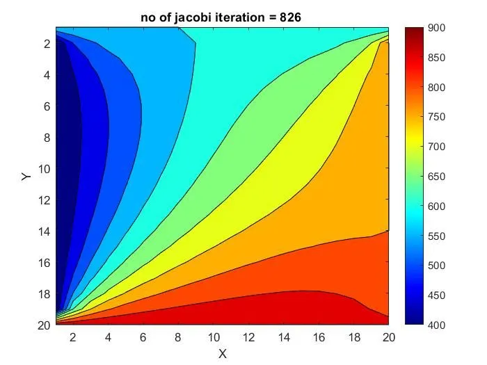
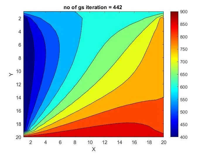
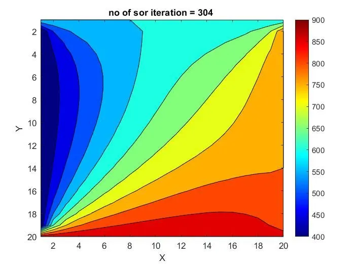
From the above plots we can see that Jacobi iterative solver takes more time and more iteration when compared with Gauss Seidel and SOR iterative solver.This is because in Jacobi method we take old values at old time steps to calculate values at next time step,whereas,in Gauss seidel method the previously calculated gets simultaneously added into next iteration.In SOR method we use some relaxation factor to multiply with our previously computed value .As we are multiplying this helps to get solution converge faster.

Transient 2D Heat Conduction(Explicit Scheme)-

clear all
close all
clc
nx=20;
ny=nx;
x=linspace(0,1,nx);
y=x;
dx=x(2)-x(1);
dy=dx;
%INITIAL CONDITIONS
T=ones(nx);
T(:,1)=400;
T(:,nx)=800;
T(1,:)=600;
T(ny,:)=900;
dt=4e-4;
alpha =1.2;
k1=alpha*(dt/dx^2);
k2=k1;
Told = T;
iter=0;
tolerance = 1e-4;
error = 9e9;
for n=1:1500 %Time loop
    for i=2:nx-1 %Space loop
     for j=2:ny-1
         term1 = k1*(Told(i+1,j)-2*Told(i,j)+Told(i-1,j));
         term2 = k2*(Told(i,j+1)-2*Told(i,j)+Told(i,j-1));
         T(i,j)= Told(i,j)+term1+term2;
     end
    end
     Told = T; %Updating
     iter = 1+iter;
end
%Plotting
contourf(T);
colormap(jet);
colorbar;
set(gca,'YDir','reverse')
title('Expicit Transient 2D Heat Conduction');
xlabel('X')
ylabel('Y')

Output-

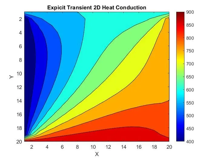
As explicit is fixed time step method,we can see by giving fixed number of time step,we have reached the convergence.As it is a fixed step ,this is a faster method than implicit method.

Transient 2D Heat Conduction(Implicit Scheme)-

Main Code-

clear all
close all
clc
nx=10;
ny=nx;
x=linspace(0,1,nx);
y=linspace(0,1,ny);
dx=x(2)-x(1);
dy=y(2)-y(1);
alpha =1.1;
dt=1e-3;
k1=alpha*(dt/(dx^2));
k2=alpha*(dt/(dy^2));
T=300*ones(nx);
T(:,1) = 400;
T(:,nx)= 800;
T(1,:) = 600;
T(nx,:)= 900;
tolerance = 1e-4;
Told=T;
T_initial=T;

%JACOBI IMPLICIT ITERATION

[T,j_iter]= jacobi_transient_function(nx,ny,k1,k2,T,tolerance,T_initial,Told);
figure(1)
 contourf(T);
colormap(jet);
colorbar;
set(gca,'YDir','reverse')
title(sprintf('No Of jacobi Iteration = %d ',j_iter));
xlabel('X')
ylabel('Y')

%GAUSS SEIDEL IMPLICIT TRANSIENT

[T,gs_iter]= gauss_seidel_transient_function(nx,ny,k1,k2,T,tolerance,T_initial,Told);
figure(2)
contourf(T);
colormap(jet);
colorbar;
set(gca,'YDir','reverse')
title(sprintf('No Of gs Iteration = %d ',gs_iter));
xlabel('X')
ylabel('Y')

%SOR IMPLICIT TRANSIENT

[T,sor_iter]= sor_transient_function(nx,ny,k1,k2,T,tolerance,T_initial,Told);
 figure(3)
contourf(T);
colormap(jet);
colorbar;
set(gca,'YDir','reverse')
title(sprintf('No Of sor Iteration = %d ',sor_iter));
xlabel('X')
ylabel('Y')
               

Jacobi Transient function-

function[T,j_iter]= jacobi_transient_function(nx,ny,k1,k2,T,tolerance,T_initial,Told)
j_iter = 0;        
for k =1:1500
    j_error = 9e9;
 while (j_error > tolerance)
    for i=2:nx-1
     for j=2:ny-1
         term1=1/(1+(2*k1)+(2*k2));
         term2=k1*term1;
         term3=k2*term1;
         H=(Told(i+1,j))+(Told(i-1,j));
         V=(Told(i,j+1))+(Told(i,j-1));
         T(i,j)= (T_initial(i,j)*term1)+(term2*H)+(term3*V);
     end
    end
    j_error =max(max(abs(Told - T)));
     Told = T;
     j_iter = 1+j_iter;
 end
 T_initial=T;
end

Gauss Siedel Transient Function-

function [T,gs_iter]= gauss_seidel_transient_function(nx,ny,k1,k2,T,tolerance,T_initial,Told )
gs_iter=0;
for n=1:1500
    gs_error = 9e9;
    while (gs_error>tolerance)
        for i=2:nx-1
            for j=2:ny-1
                term1=1/(1+(2*k1)+(2*k2));
         term2=k1*term1;
         term3=k2*term1;
         H=(Told(i+1,j))+(T(i-1,j));
         V=(Told(i,j+1))+(T(i,j-1));
         T(i,j)= (T_initial(i,j)*term1)+(term2*H)+(term3*V);
            end
        end
       gs_error=max(max(abs(Told-T)));
                Told=T;
                gs_iter=gs_iter+1;
    end
    T_initial = T;
end

SOR Transient Function-

function[T,sor_iter]= sor_transient_function(nx,ny,k1,k2,T,tolerance,T_initial,Told )
sor_iter=0;
omega = 1.1;
for n=1:1500
    sor_error = 9e9;
    while sor_error>tolerance
        for i= 2:nx-1
            for j=2:ny-1
                       term1=1/(1+(2*k1)+(2*k2));
         term2=k1*term1;
         term3=k2*term1;
         H=(Told(i+1,j))+(T(i-1,j));
         V=(Told(i,j+1))+(T(i,j-1));
         
            T(i,j)=((1-omega)*Told(i,j))+(omega*((T_initial(i,j)*term1)+(term2*H)+(term3*V)));
            end
        end
        sor_error=max(max(abs(Told-T)));
        Told = T;
        sor_iter=sor_iter+1;
    end
    T_initial =T;
end

Outputs-

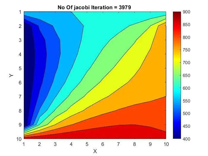
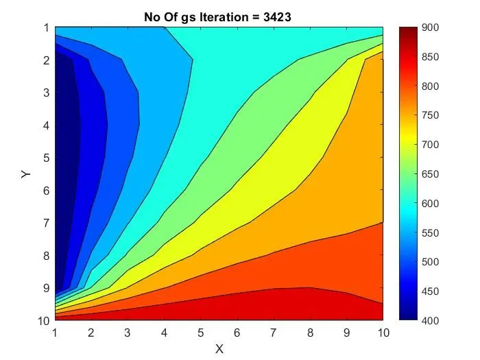
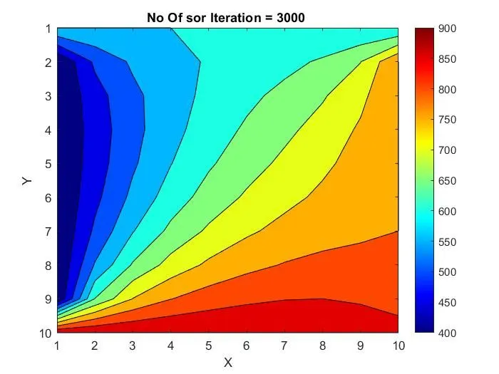
From the above plots we can clearly see that number of iterations required by each iterative method is of order of

Jacobi method > Gauss Seidel method > SOR method.

This is because of the way each method takes the information for each iteration.Jacobi uses old values to run next iteration while,Gauss Seidel uses simultaneouslly uses info from previous and next step to run the iterations.And SOR uses relaxation factor to reduce convergence steps.