Week 11 - Simulation of Flow through a pipe in OpenFoam
Aim -
1.To simulate flow through a costant cross section circular pipe by applying wedge boundry condition using icoFoam solver.
2.To validate the results with Hagen-Poiseuille's equations for a fully developed flow.
3.To write a code MATLAB to automate the generation of blockMeshDict file for the circular pipe
Introduction -
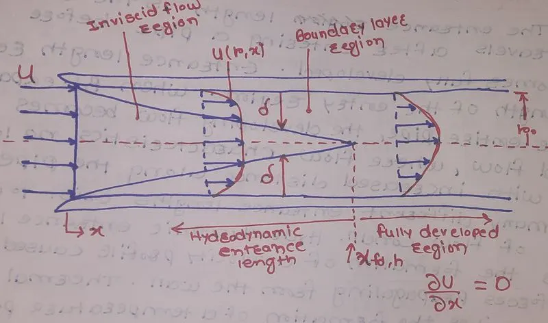
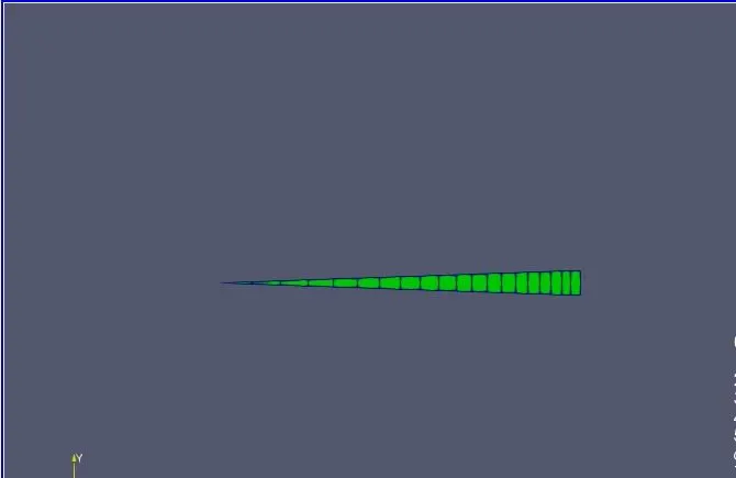
Consider a incompressible laminar and newtonian flow through a pipe having constant circular cross section throughout the length(Hagen Poiseuille flow).The basic model geometry is shown in figure above.The diameter of the pipe D = 0.03m and length of the pipe L= 5m and water is the working fluid. First we need to generate the blockmesh dict file,which is later used by openfoam to generate the mesh.Then we need to use the above generated file to set up the physical model and run the simulation using OpenFoam.Geomety,loadings,boundary conditions and materials are symmetric with respect to z axis,thus ,the flow has axisymmetric nature.The suitable wedge angle(<5') is considered.
So in the results we need to observe the change in velocity profile and pressure drop across the length of the pipe. We also need to calculate the magnitude of shear stress acting on the walls of the domian.At last,validate results with analytical solution obtained from Hagen Poiseullle equation. Assume constant velocity inlet and constant zero gauge pressure outlet as the initial boundary condition.
The following data is provided,
1. Reynolds Number ( Re) = 2100
2. Wedge Angle (`theta` ) = 4 degrees
3. Diameter of the Pipe (D) = 0.03 m
4. Outlet Gauge Pressure (`P_o`) = 0 Pa
5. Temperature of the Working Fluid (T) = 20 degreeCelcius
6. Dynamic Viscosity of Water ( `mu`) = 0.997 * 10^-3 Pa.sec
7. Kinematic Viscosity (`nu` ) = 1 * 10^-6 m^2/sec
Theory -
Hagen-Poiseuille Law(H-P Law) :
In nonideal fluid dynamics,the Hagen Poiseuille equation also known as Poiseuille law,is a
physical law that gives the pressure drop in an incompressibe and newtonian fluid in laminar flow flowing through a long
cylindrical pipe of constant cross section.
The assumptions of the equations are that the fluid is incompressible and Newtonian and that the flow is laminar
through a pipe of constant circular cross section that is substantially longer than it's diameter and there is no accceleration of fluid in the pipe.H-P Law is valid only in hydrodynamically fully developed region i.e only after the entrance region.
Entrance Region :
The length of the entrance is the distance that fluid travels after entering a pipe before full
development of the flow.Entrance length refers to the entry region.When the boundary layer expands to fill the entire pipe,
the developing flow becomes fully developed flow,where flow characteristics no longer change with increased distance along the pipe.
Many different entrance lengths exist to describe a variety of flow conditions.Hydrodynamic entrance length describes the formation of a velocity profile caused by viscous forces proagating from the wall.Thermal entrance region describes the formation of a temperature profile.Awareness of entrance length may be necesssary for the effective placement of the instrumentations such as fluid flow meters.
Hydrodynamic entrance length for a laminar flow is given by,
Le_laminar = 0.05.Re.D
Fully Developed Region :
The region beyond the enrance region beyond the entrance region in which the velocity profile is fully developed and remains unchanged is called hydrodynamically fully developed region.The flow is said to be fully developed
when normalized temperature and velocity profile remains unchanged across the length.The velocity still varies in the radial
direction(velocity gradient),but remains constant across the axial direction.
The velocity profile in the fully developed region is parabolic in laminar flow amd somewhat flatter or fuller in turbulent flow due to eddy motion and more vigorous mixing in the radial direction.The time averaged velocity profile remains unchanged when the flow is fully developed.It can be shown mathematically as,
delU(r,x)/delx = 0 = U = U(r)
Calculations for Analytical Solution -
1). Average Velocity or Inlet Velocity :
`Re = rho.D.(V_(avg))/mu`
`2100 = 997*0.03*V_(avg)/0.997*10^-3`
`V_(avg) = 0.07 m/s`
2). Maximum Velocity or Velocity at Fully Developed Region :
`V_max = 2.V_(avg)(1-r^2/R^2)`
where at boundary r=R.
For fully developed flow maximum velocity will be at r=0,
Thus,
`V_max = 2.V_(avg`
`V_max = 2*0.07`
`V_max = 0.14 m/s`
3). Hydraulic Entrance Length :
`(Le)_(laminar) = 0.05.Re.D`
`(Le)_(laminar) = 0.05*2100*0.03`
`(Le)_(laminar) = 3.15 m`
As fully developed region is after the length of Le = 3.15 m ,lets assum the length of pipe as = 5 m.
4). Length of fully developed region (`L_(fdr`) :
`L_(fdr )= L_T - L_e`
`L_(fdr = 5 - 3.15`
`L_(fdr = 1.85 m`
According to Darcy Weisbach equation,The Friction factor for laminar flow is,
`f = 64/R_e`
`f = 64/2100`
`f = 0.0305`
5). Pressure drop across the fully developed region(`Delta P`) :
`Delta P = 32*0.07*0.997*10^-3*1.85/0.03^2`
`Delta P = 4.594 Pa`
6). Kinematic Pressure Drop(Delta P_k) :
`Delta P_k = (Delta P)/rho`
`Delta P_k = 4.594/997`
`Delta P_k = 0.004607`
Shear Stress :
When the fluid is in motion ,shear stresses are developed due to the particle in the fluid moving relative to
each other.For a fluid moving in a pipe,the velocity will be zero at the wall and it will increase while moving towards the
center of the pipe.Shear force is present due to the movement of adjacent fluid layers at different velocities.Fluid obeying
the Newton's law,where values of dynamic viscosity(`mu`) are constant are known as Newtonian Fluids.If `mu` is constant the shear stresses are relatively dependent on the velocity gradient.
Wall Shear Stress(`tau_omega`),
`tau_omega = f/4.rho.V_(avg)^2/2`
`tau_omega = 0.0305*997*0.07^2/8`
`tau_omega = 0.0186 Pa`
Geometry Creation and Applying Boundry Conditions -
The blockMesh utility is used to-
* create geometry by building blocks from the co-ordinates of their vertices.
* generate a structured mesh by defining the number of nodes for each main direction.
* create the patches for each of the boundary conditions.
Matlab Code To Generate blockMeshDict File :
Main Code
close all
clear all
clc
L = 5;                  %Length of pipe
theta = 2;              %Angle of wedge wrt axis
r = 0.015;              %Radius of pipe
rho = 997;              %Density of working fluid
Re =2100;               %Reynolds number
sf = 1;                  %Scaling factor
sgx = 0.3;              %Simple grading along X-direction
sgy = 1;                %Simple grading along Y-direction
sgz = 1;                %Simple grading along Z-direction
dx = 20;                %Number of cells in X-direction
dy = 1;                 %Number of cells in Y-direction
dz = 500;               %Number of cells in Z-direction

blockMeshdict_script_function(sf,L,r,theta,dx,dy,dz,sgx,sgy,sgz)
Function:
function blockMeshdict_script_function(sf,L,r,theta,dx,dy,dz,sgx,sgy,sgz ...
    )
x1 = r*cosd(theta);
y1 = r*sind(theta);
z1 = 0;
x2 = r*cosd(360-theta);
y2 = r*sind(360-theta);
z2 = L;
 % Header lines
 line1='/*--------------------------------*-C++ -*--------------------------------*';
 line2='  =========                 |                                               ';
 line3='        /  F ield         |  OpenFOAM: The Open Source CFD Toolbox        ';
 line4='       /   O peration     |  Website: https://openfoam.org                ';
 line5='      /    A nd           |  Version: 8                                   ';
 line6='     /     M anipulation  |                                               ';
 line7='*-------------------------------------------------------------------------*/';
 line8='FoamFile';
 line9='// * * * * * * * * * * * * * * * * * * * * * * * * * * * * * * * * * * * * * //';

 % BlockMeshDict
 f=fopen('blockMeshDict','w');
 fprintf(f,'%s\n',line1,line2,line3,line4,line5,line6,line7,line8);
 fprintf(f,'{\n');
 fprintf(f,'\tversion\t\t 2.0;\n\tformat \t\tascii;\n\tclass\t\tdictionary;\n\tobject\t\tblockMeshDict;\n}\n');
 % Starting Line
 fprintf(f,'%s',line9);
 % Scaling Factor
 fprintf(f,'\n\nconvertToMeters     %d;\n\n',sf);
 % Vertices
 fprintf(f,'vertices\n(\n\n\t(0 0 0)\n\t(%f %f %f)\n\t(%f %f %f)\n\t(0 0 %f)\n\t(%f %f %f)\n\t(%f %f %f)\n);\n',x1,y1,z1,x1,y1,z2,z2,x2,y2,z1,x2,y2,z2);
 % Blocks
 fprintf(f,'\nblocks\n(\n\thex (0 4 1 0 3 5 2 3) (%d %d %d) simpleGrading (%f %f %f)\n);\n',dx,dy,dz,sgx,sgy,sgz);
 % Edges
 fprintf(f,'\nedges\n(\n\tarc 1 4 (%f %f %f)\n\tarc 2 5 (%f %f %f)\n);\n',x1/2,y1/2,z1,x2/2,y2/2,z2);
 % Boundaries
 fprintf(f,'\nboundary\n(\n\n\taxis\n\t{\n\t\ttype empty;\n\t\tfaces\n\t\t(\n\t\t\t(0 3 3 0)\n\t\t);\n\t}\n');
 fprintf(f,'\tinlet\n\t{\n\t\ttype patch;\n\t\tfaces\n\t\t(\n\t\t\t(0 4 1 0)\n\t\t);\n\t}\n');
 fprintf(f,'\toutlet\n\t{\n\t\ttype patch;\n\t\tfaces\n\t\t(\n\t\t\t(3 5 2 3)\n\t\t);\n\t}\n');
 fprintf(f,'\tleftwall\n\t{\n\t\ttype wedge;\n\t\tfaces\n\t\t(\n\t\t\t(4 0 3 5)\n\t\t);\n\t}\n');
 fprintf(f,'\trightwall\n\t{\n\t\ttype wedge;\n\t\tfaces\n\t\t(\n\t\t\t(0 1 2 3)\n\t\t);\n\t}\n');
 fprintf(f,'\touterwall\n\t{\n\t\ttype wall;\n\t\tfaces\n\t\t(\n\t\t\t(1 4 5 2)\n\t\t);\n\t}\n\n\n);\n');
 % Patch Pairs
 fprintf(f,'\nmergePatchPairs\n(\n);\n');
 % Ending Line
 fprintf(f,'\n%s',line9);
 fclose(f);
end
Output blockMeshDict file
/*--------------------------------*-C++ -*--------------------------------*
  =========                 |
        /  F ield         |  OpenFOAM: The Open Source CFD Toolbox
       /   O peration     |  Website: https://openfoam.org
      /    A nd           |  Version: 8
     /     M anipulation  |
*-------------------------------------------------------------------------*/
FoamFile
{
	version		 2.0;
	format 		ascii;
	class		dictionary;
	object		blockMeshDict;
}
// * * * * * * * * * * * * * * * * * * * * * * * * * * * * * * * * * * * * * //

convertToMeters     1;

vertices
(

	(0 0 0)
	(0.014991 0.000523 0.000000)
	(0.014991 0.000523 5.000000)
	(0 0 5.000000)
	(0.014991 -0.000523 0.000000)
	(0.014991 -0.000523 5.000000)
);

blocks
(
	hex (0 4 1 0 3 5 2 3) (20 1 500) simpleGrading (0.300000 1.000000 1.000000)
);

edges
(
	arc 1 4 (0.007495 0.000262 0.000000)
	arc 2 5 (0.007495 -0.000262 5.000000)
);

boundary
(

	axis
	{
		type empty;
		faces
		(
			(0 3 3 0)
		);
	}
	inlet
	{
		type patch;
		faces
		(
			(0 4 1 0)
		);
	}
	outlet
	{
		type patch;
		faces
		(
			(3 5 2 3)
		);
	}
	leftwall
	{
		type wedge;
		faces
		(
			(4 0 3 5)
		);
	}
	rightwall
	{
		type wedge;
		faces
		(
			(0 1 2 3)
		);
	}
	outerwall
	{
		type wall;
		faces
		(
			(1 4 5 2)
		);
	}


);

mergePatchPairs
(
);

// * * * * * * * * * * * * * * * * * * * * * * * * * * * * * * * * * * * * * //
Choosing the Solver :
To simulate the the given problem,we first need to choose the appropriate openfoam tutorial,that suits our problem statement.I chose icoFoam solver,under incompressible tutorials.icoFoam is a PISO loop based solver.It is a transient laminar incompressible solver.The flow will therefore be solved transiently until the steady state is obtained.
Calculating Time Step Size :
While selecting numerical schemes to solve the discretized governing equations,the only accuracy is not enough
.Our numerical scheme should be both stable and accurate.We say the numeriacal scheme is stable when the truncation error does not increase after each timestep.So there exist a stability criteria that calculates the extreme values of space and time step for such numerical schemes to attain stability,we use CFL stability criteria to get our stability codition.
The courant number is by defination a local variable therefore,depending on the velocity field and mesh size,we have a field of CFL variable.Time step is calculated over each cell with the help of CFL criteria.
`CFL(C) = (DeltaT*U)/dx`
where, `DeltaT` = Time step.
dx = Smallest cell size
U = Velocity
The flow velocity varies across the domain,and we must ensure that C<1 for every cell.To do that we have taken time step equal to 0.011.
/*--------------------------------*- C++ -*----------------------------------*\
  =========                 |
  \\      /  F ield         | OpenFOAM: The Open Source CFD Toolbox
   \\    /   O peration     | Website:  https://openfoam.org
    \\  /    A nd           | Version:  9
     \\/     M anipulation  |
\*---------------------------------------------------------------------------*/
FoamFile
{
    format      ascii;
    class       dictionary;
    location    "system";
    object      controlDict;
}
// * * * * * * * * * * * * * * * * * * * * * * * * * * * * * * * * * * * * * //

application     icoFoam;

startFrom       startTime;

startTime       0;

stopAt          endTime;

endTime         80;

deltaT          0.011;

writeControl    timeStep;

writeInterval   50;

purgeWrite      0;

writeFormat     ascii;

writePrecision  6;

writeCompression off;

timeFormat      general;

timePrecision   6;

runTimeModifiable true;


// ************************************************************************* //
Initial And Boundary Conditions -
Initial Velocity Condition :
/*--------------------------------*- C++ -*----------------------------------*\
  =========                 |
  \\      /  F ield         | OpenFOAM: The Open Source CFD Toolbox
   \\    /   O peration     | Website:  https://openfoam.org
    \\  /    A nd           | Version:  9
     \\/     M anipulation  |
\*---------------------------------------------------------------------------*/
FoamFile
{
    format      ascii;
    class       volVectorField;
    object      U;
}
// * * * * * * * * * * * * * * * * * * * * * * * * * * * * * * * * * * * * * //

dimensions      [0 1 -1 0 0 0 0];

internalField   uniform (0 0 0);

boundaryField
{
    outlet
    {
    	type		zeroGradient;
    }
    inlet
    {
        type            fixedValue;
        value           uniform (0 0 0.070000);
    }

    axis
    {
        type           empty;
    }

  leftwall
    {
        type           wedge;
    }
    rightwall
    {
        type           wedge;
    }
    outerwall
    {
        type         noSlip;
    }
}

// ************************************************************************* //
Pressure Condition :
/*--------------------------------*- C++ -*----------------------------------*\
  =========                 |
  \\      /  F ield         | OpenFOAM: The Open Source CFD Toolbox
   \\    /   O peration     | Website:  https://openfoam.org
    \\  /    A nd           | Version:  9
     \\/     M anipulation  |
\*---------------------------------------------------------------------------*/
FoamFile
{
    format      ascii;
    class       volScalarField;
    object      p;
}
// * * * * * * * * * * * * * * * * * * * * * * * * * * * * * * * * * * * * * //

dimensions      [0 2 -2 0 0 0 0];

internalField   uniform 0;

boundaryField
{
    inlet
    {
    	type		zeroGradient;
    }
  outlet
    {
        type            fixedValue;
        value           uniform 0;
    }

    axis
    {
        type           empty;
    }

  leftwall
    {
        type           wedge;
    }
    rightwall
    {
        type           wedge;
    }
    outerwall
    {
        type         zeroGradient;
    }
}

// ************************************************************************* //
Physical Properties :
The physical parameters for the specific flow problem are described in the file called TransportProperties file.This file is
located in the constant directory.In our case, we assume that our fluid is water and kinematic viscosity of water is given
as 1e-6 m^2/sec.This file will be same for all analysis with different grading factor.
/*--------------------------------*- C++ -*----------------------------------*\
  =========                 |
  \\      /  F ield         | OpenFOAM: The Open Source CFD Toolbox
   \\    /   O peration     | Website:  https://openfoam.org
    \\  /    A nd           | Version:  9
     \\/     M anipulation  |
\*---------------------------------------------------------------------------*/
FoamFile
{
    format      ascii;
    class       dictionary;
    location    "constant";
    object      transportProperties;
}
// * * * * * * * * * * * * * * * * * * * * * * * * * * * * * * * * * * * * * //

nu              [0 2 -1 0 0 0 0] 0.000001;


// ************************************************************************* //
Post Processing -
The primary post processing tool provided with OpenFoam is ParaView.The results that are written in the time directories
can be viewed using ParaView.To launch ParaView a command called paraFoam is used from within the case directory. paraFoam is a script file, which launches ParaView.
Mesh Stretching or Mesh Refinement :
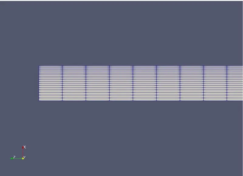
Now to capture the boundary layer effect it is necessary to use finer mesh near the walls.The process of changing mesh,
according to the physical need of the problem,in order to produce more accurate results, is called as mesh refinement.We
are going to make our mesh finer near the wall by using non-zero grading factors in the blockMeshDict file known as simple
grading.For our problem we are going to take grading factor of 0.3.
Results -
Below are the data extracted for shear stress,maximum velocity and pressure drop from paraview using probe location command.
The values are extracted at 5 m and 3.15 m along pipe length.

Fig : Maximum Velocity and Pressure Drop
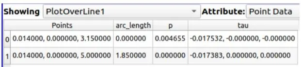
Fig : Wall Shear Stress
Maximum Velocity(`V_max`) = 0.138 m/s
Pressure Drop (`DeltaP`) = 0.004655 Pa
Wall Shear Stress (`tau_omega`) = 0.0175
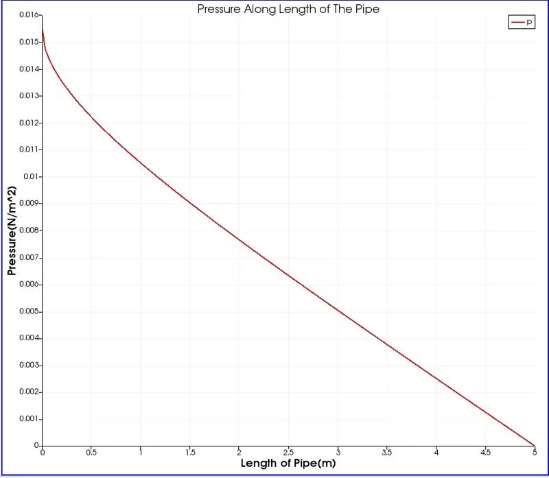
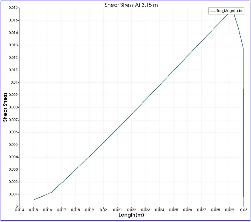
Fig. -Pressure Drop Along the Length Of Pipe Fig.- Shear Stress At 3.15 m(at start of fully developed region)
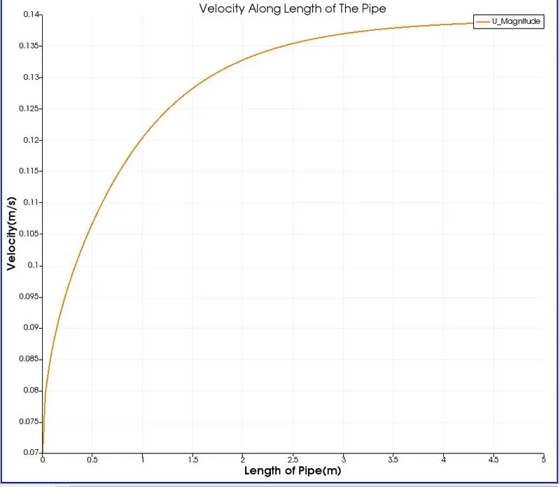
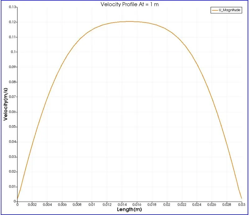
Fig. - Velocity Along the Length of Pipe Fig. - Velocity Profile At 1m
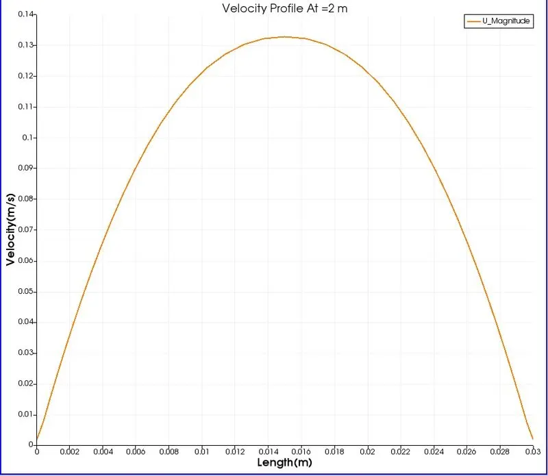
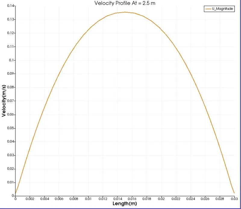
Fig. - Velocity Profile At 2 m Fig. - Velocity Profile At 2.5 m
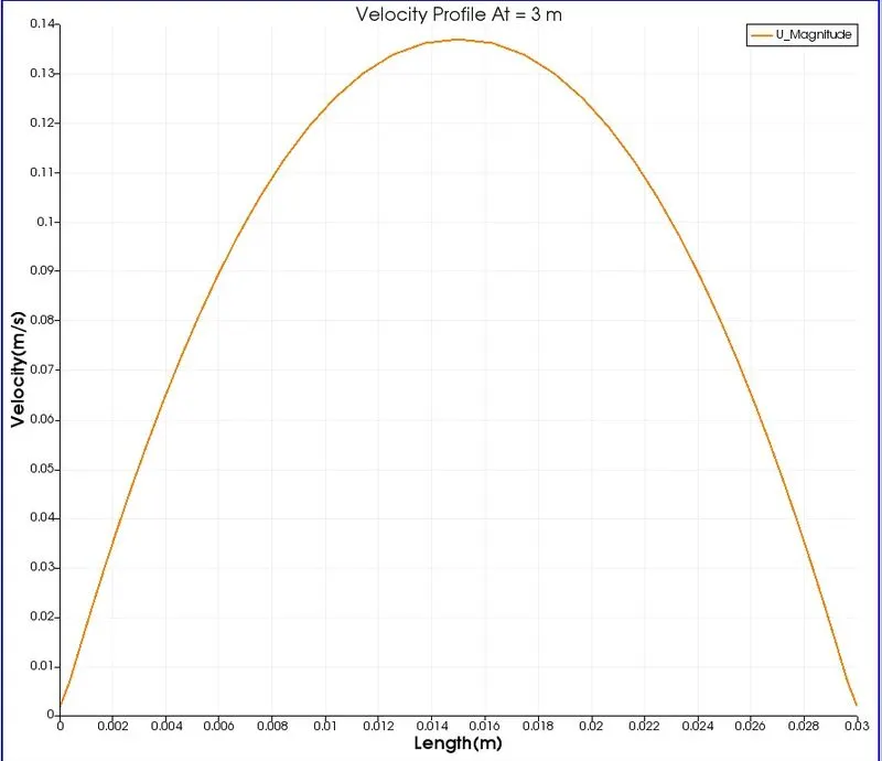
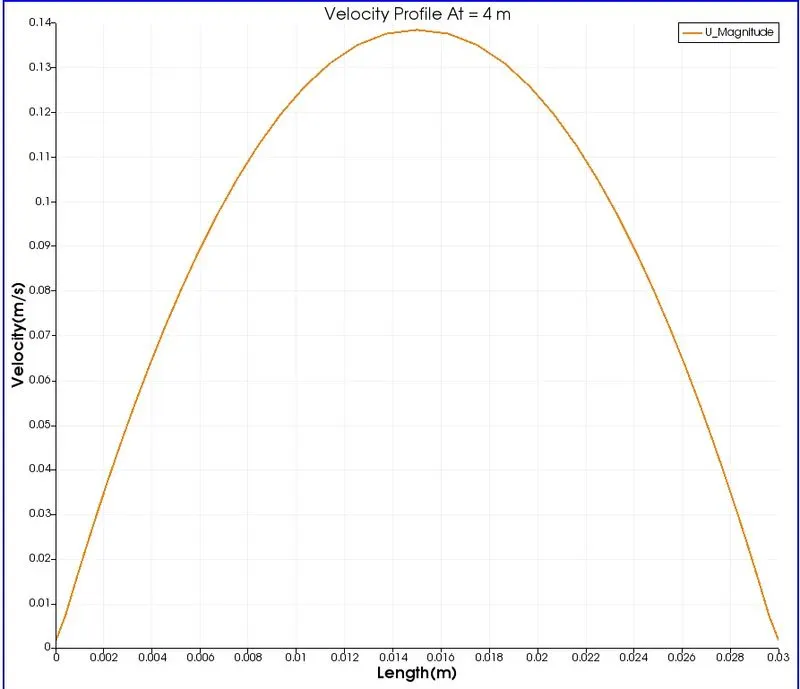
Fig. - Velocity Profile At 3m Fig. - Velocity Profile At 4 m
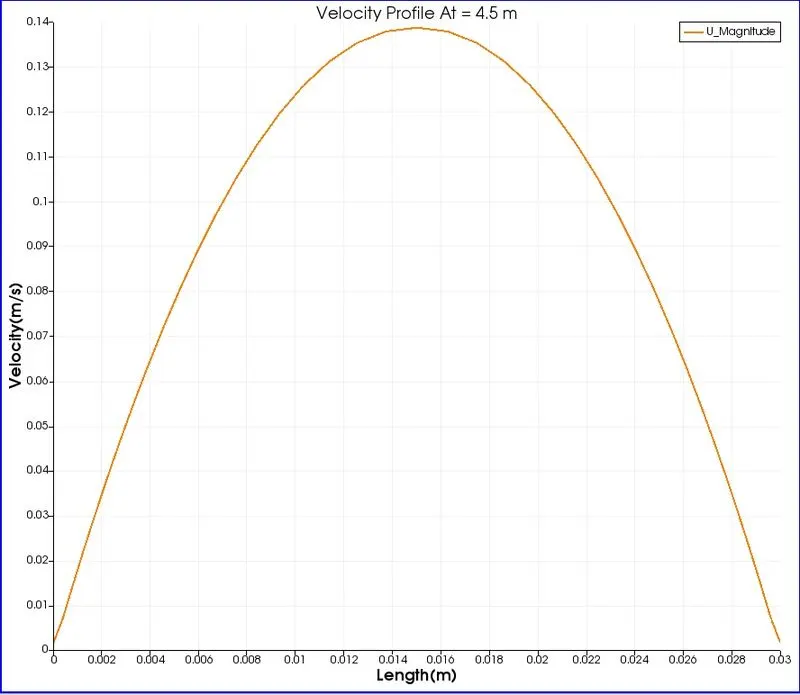
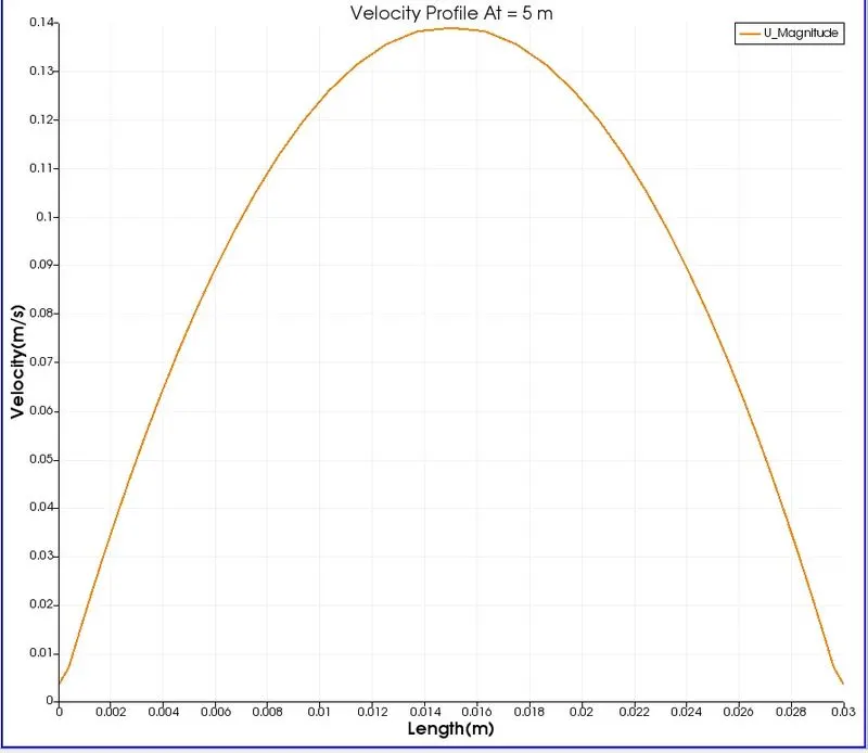
Fig. - Velocity Profile At 4.5 m Fig. - Velocity Profile At 5 m
We can see from the above plots that upto around 3.15 m velocity profile changes but after that it remains constant,which validates with our analytical hydrodynamic entrance length of 3.15 m as per Hagen-Poiseuille's equations.
Comparison Of Analytical & Numerial Results -
| Analytical Solution | Numerical Solution | Error | |
| 1). Maximum velocity(`V_max`) | 0.14 | 0.138 | 0.002 |
| 2). Pressure Drop(`DeltaP`) | 0.00460 | 0.00465 | -0.00005 |
| 3). Wall Shear Stress(`tau_omega`) | 0.0186 | 0.0175 | 0.0011 |
Conclusion -
1) As we can see from the graphs ,the velocity profile remains almost unchanged after 3.15 m and thus satisfies with fully developed region value calculated from Hagen-Poiseuilles equations.
2) Also numerical values extracted from paraView data are found to be close to analytical values.
3) Numerical Hydrodynamic length validates with analytical value.
4) Velocity profiles obtain at different lenghts along the pipe closely resembles theoretical profile bt Hagen_Poiseullie' Law.
5)Wall shear stress in the fully devloped region increases as the we move away from the center of the pipe and vice versa.
6) Thus the Hagen-Poiseuille's equations for circular pipe with constant cross section are verified through numerical simulation of laminar flow through pipe.