Week 7: Shock tube simulation project
1] AIM :
Perform transient shock tube simulation using Converge CFD.
2] OBJECTIVE :
*Simulate the propagation of shock waves through a shock tube.
*Plot temperature and pressure history in the entire domain.
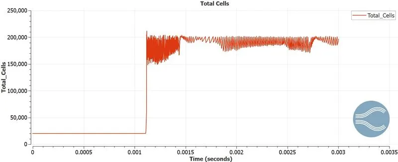
*Plot the cells as a function of time.
3] INTRODUCTION AND THEORY :
A shock tube in its simplest form is a long tube with closed ends separated into two sections, namely, the driver section and the drivensection, usually by a diaphragm.During a shock wave experiment the driven (low-pressure) section of the shock tube is filled with the test gas mixture, and the driver section is overpressured with gas, often helium or a helium mixture, until the diaphragm bursts. An incident shock wave quickly forms and travels rapidly ahead of the driver gas into the driven section, increasing the temperature and pressure of the test gas behind it. On reaching the end wall of the shock tube, this incident shock wave reflects from the wall and propagates back toward the driver section, stagnating and further compressing and heating the test gas to its initial prereaction temperature and pressure.
One operational drawback of conventional shock tube experiment is the single-shot nature of the facility.Applications of shock
tube have also been extended to combustion studies in condensed or mixed phases, such as in aerosols. Earlier experimental studies mostly concentrated on measurements of shock-aerosol interactions, evaporation and ignition of single droplets, and ignition properties of diesel-injector-generated sprays.
The sudden expansion of a gas at high pressure into a gas at low pressure produces a plane shock wave that then propagates through a long closed tube. The shock wave is used to produce a rapid increase in the pressure and the temperature of a reactive mixture. In most shock tubes, the shock wave is reflected at the end of the tube and produces during its way back a second rise in temperature. This technique is mainly used to study elementary steps, as well as pyrolysis and high-temperature autoignition in very dilute mixtures.
4] SOLUTION PROCEDURE :
To perform this simulation ,we will follow the below procedure :-
Geometry Creation --> Case Setup --> Solution --> Post Processing
4.1] GEOMETRY CREATION :
* Launch Converge and start a new project.
*Import the give .stl file.
*The dimensions of the tube are = 0.2 * 0.01 * 0.01 m
*Upon running a diagnosis check,it was noted that there were some non-manifold edge problems.This was due to presence of diaphragm inside the tube.This was deleted for this analysis and this resolves the non-manifold edge problem.
* In converge ,geometries are represented as triangles.So we need to group these triangles to create boundaries.This is the
fundamental step in Converge.
Geometery => Boundary => Flag => click on add and add 1 boundaries => rename first boundary as high_pressure & select triangles from the half side of the geometry as shown =>apply.
*Simillarly create low pressure region.
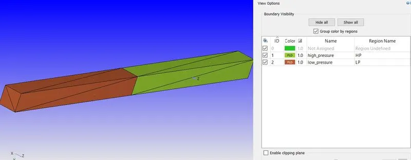
* As our flow is internal,we want all the normals to point into the fluid domain.To do that,
click on normal toggle => transform => normal => click on triangle with outside pointing normal => apply
* Make sure that geometry is clean,
Diagnosis => find => no errors.
4.2] CASE SETUP :
* Click on Begin Case Setup => General Flow => Done.
* Our working fluid will be air .
* Materials => Predefined mixture => Air => uncheck reaction mechanism => check species => Apply & Done.
* Keep default global transport parameters.
* In species add oxygen and nitrogen.
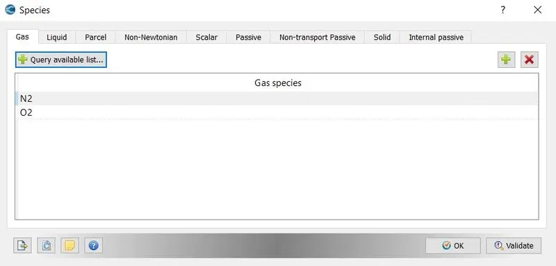
* We will be running transient simulation.To set this follow below steps,
Run Parameters => Solver => select transient solver => simulation mode full hydrodynamic => Gas flow solver compressible.
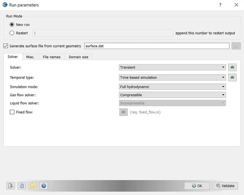
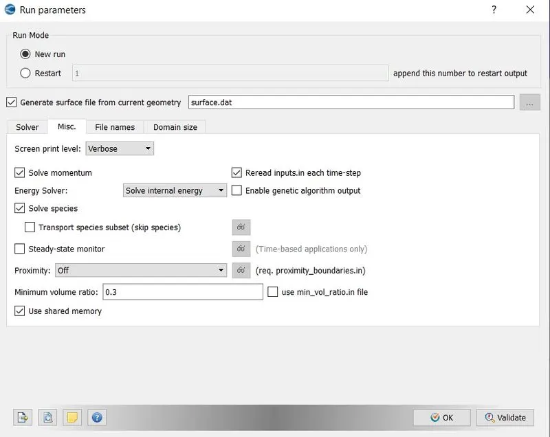
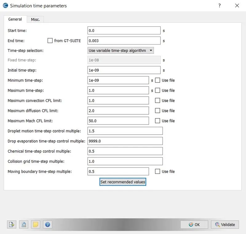
*4.2.1] SIMULATION TIME PARAMETERS =>
Start Time - 0 sec
End Time - 0.003 sec
Initial Time Step - 1e-9 sec.
Minimum Time Step - 1e-9 sec.
Maximum time step - 1 sec.
Maximum Convection CFL limit - 1.0.
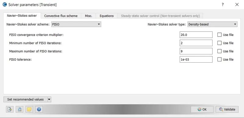
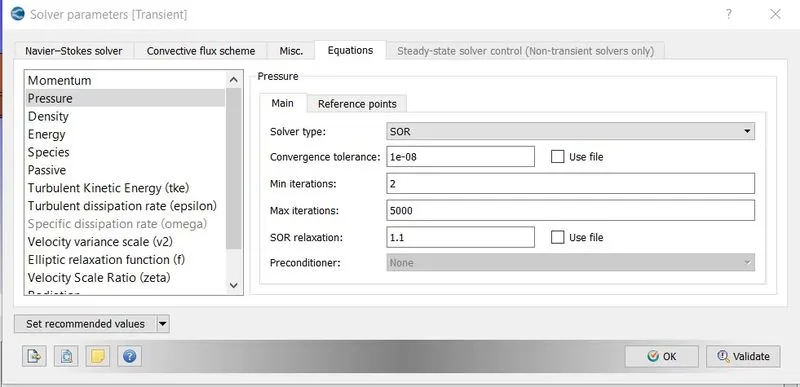
*4.2.2] SOLVER PARAMEETERS =>
Navier-Stokes solver Scheme => PISO
Navier-Stokes solver Type => Density Based
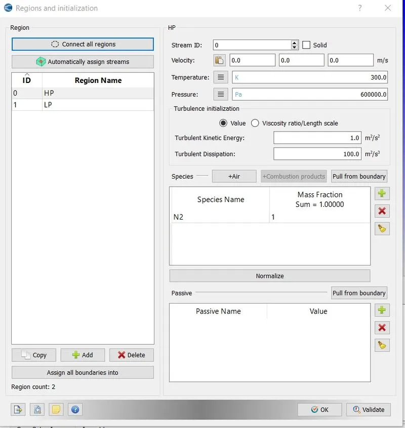
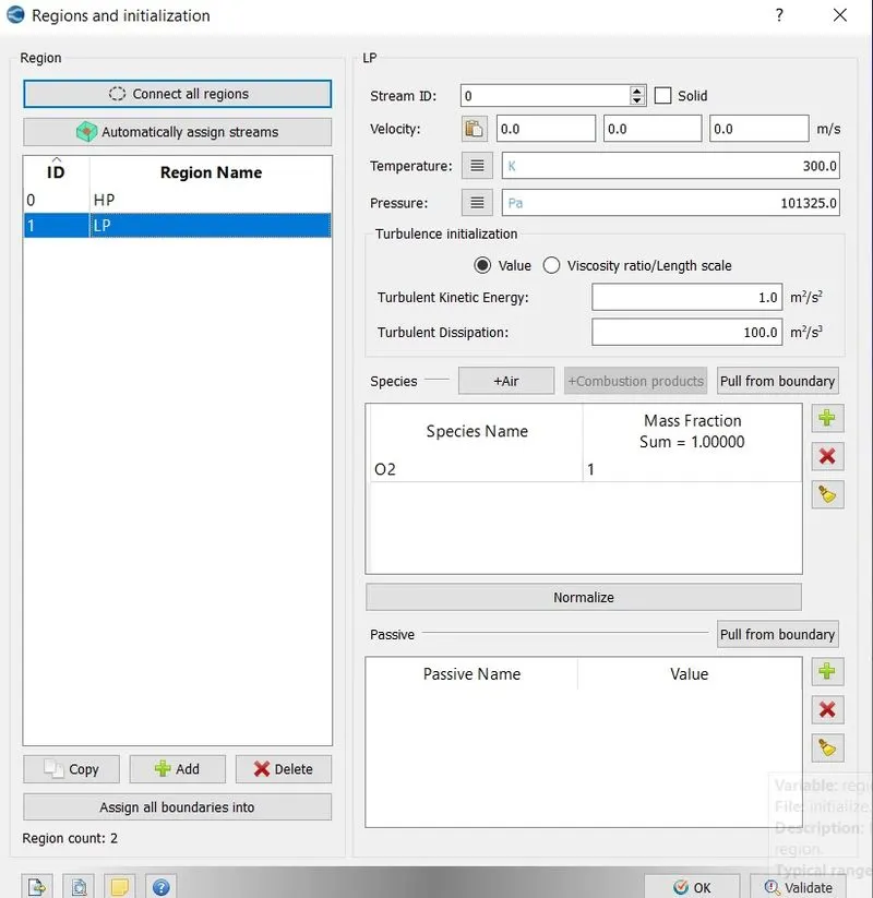
* Now before setting the boundaries,set initial region and set initial pressure and define air species.This region will be
assigned to each boundary.
*4.2.3] BOUNDARIES =>
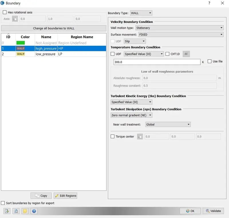
high_pressure -
Boundary Type -WALL
Velocity Boundary Condition - Slip
Temperature Boundary Condition - Zero normal gradient(NE)
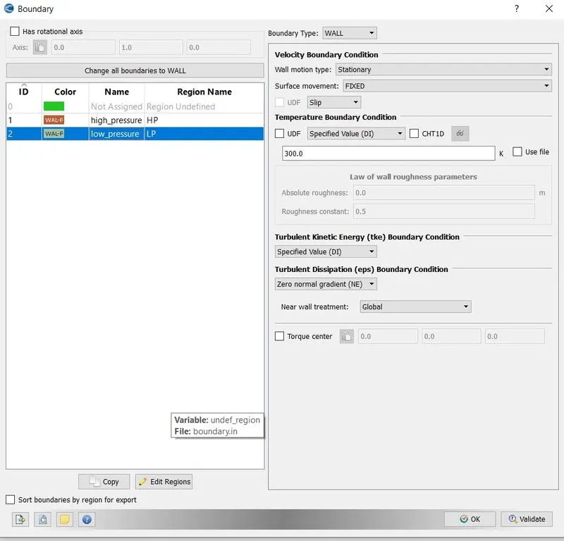
low_presssure -
Boundary Type - WALL
Velocity Boundary Condition - Slip
Temperature Boundary Condition - Zero normal gradient(NE)
* 4.2.4] EVENTS
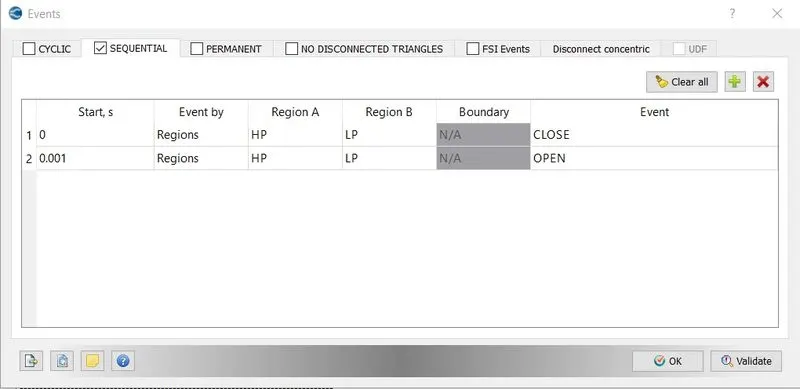
In physical world the shock tube experiment is carried out by bursting the diaphragm and allowing high pressure side to interact with low pressure side.This is not possible to simulate in virtual world.So we will set an event to tell the solver when it should permit high pressure and low pressure sides to interact.
Initial Conditions and Events => select Events => in SEQUENTIAL add two events as shown in below image => ok.
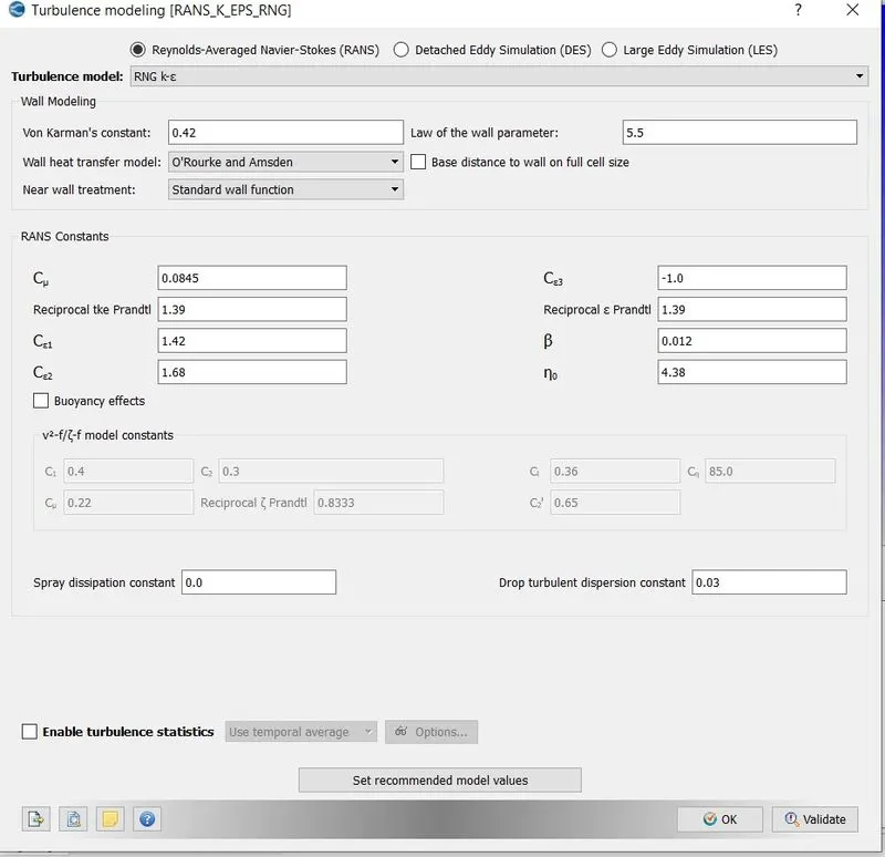
* For turbulence model select RNG k-epsilon.
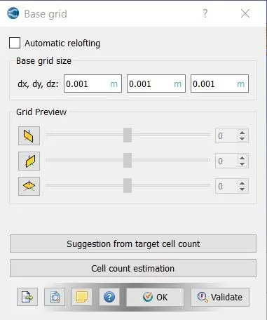
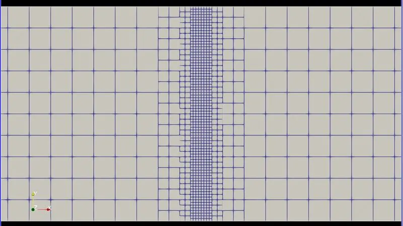
*In converge mesh generation is a fully automatic process.Converge uses cut cell method to generate the mesh.
Base Grid = dx= 0.001 ; dy = 0.001 ; dz = 0.001 => ok
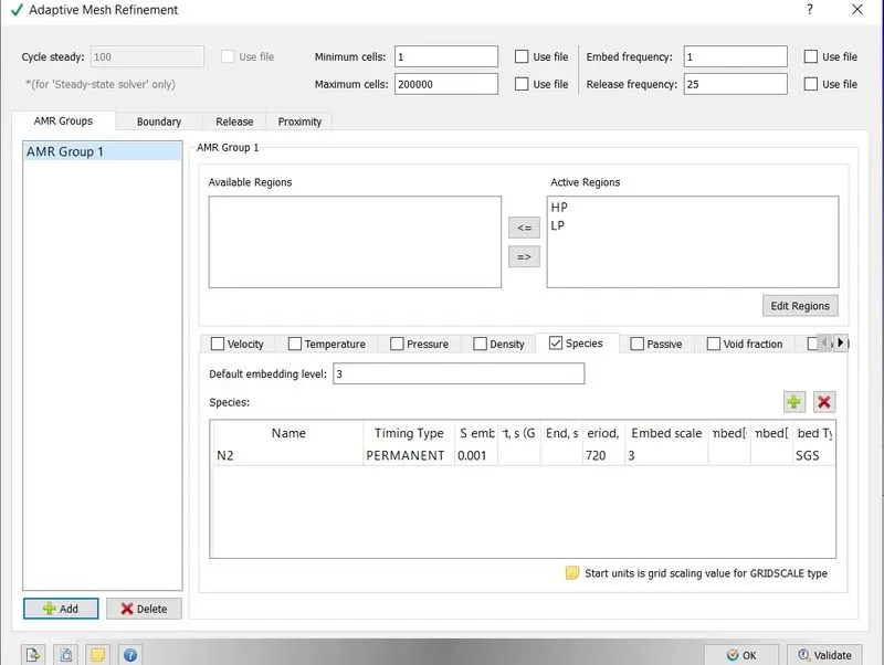
*As we want to moniter how different species behaves inside the tube,we need to refine the mesh near it.To do that we will do adaptive mesh refinement.
* 4.2.5]ADAPTIVE MESH REFINEMENT =>
Minimum Cells - 1
Maximum Cells - 200000
Active Regions - HP & LP
Check Species
Default Embedding Level -3
Species name - N2
Timing type - PERMANENT
SGS embed - 0.001
Period -720 s
Embed scale -3
Embed type - SGS
*In post variable selection,select the variables which needs to be post processed and set species mass fraction.
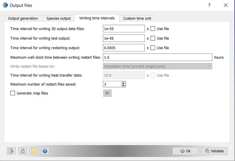
*We want our post processed graphes and animations to be smooth,so we want ample amount of ouput files.It is good practice to have at least 100 3D output files and same amount of text output files.
4.3] SOLUTION :
*For running the simulation,first we need to export all the input files to the folder where we want to save our 3D output files,
File => Export => Export Input Files => select the desired folder => Export.
*Now we will use CYGWIN command prompt to run our simulation.But before running the simulation first we need executables which will solve the simulation,for that paste mpiexec.exe and converge.exe into the folder where we have exported all our input files.
*Now using CYGWIN command prompt,navigate to the folder where all the input files are exported,and type the below command,
mpiexec.exe -n 4 converge.exe restricted </dev/null> logfile &
*In the above command ,mpiexec.exe will help us to run our simulation in parallel,-n 4 are the number of cores on which we
want to run our simulation.As we are using the version of converge which has limit on the size of the file it can solve hence the command restricted.And the last part of the command dump all the data that is being generated into the logfile, which we can access during simulation procedure to see where our simulation has reached.
*The above command will create a folder named output containing all the generated 3D output data.As we will be using paraview as the postprocessing tool.Hence we need to convert these output files into the format that paraview can read.For this we will use converge post convert tool.
Go to converge post processing 3D =>give case name => select the file type => navigate to the output folder and select it
=> select all files => select all variables => convert.
This will create group file ,which will be used by paraview to post process our results.
4.4] POST-PROCESSING :
4.4.1] MESH -

4.4.2] VELOCITY CONTOUR -

4.4.3] TEMPERATURE CONTOUR -

4.4.4] PRESSURE CONTOUR -

4.4.5] PLOTS -
4.4.6] ANIMATIONS :
Velocity -https://www.youtube.com/shorts/fbBp-TYR7Cs
Pressure -https://www.youtube.com/shorts/8aa-3RP4tUY
Temperature -https://www.youtube.com/shorts/NwyWpgIU7xc
AMR -https://www.youtube.com/watch?v=CKMJgOjxhLQ
N2 Mass Fraction -https://www.youtube.com/watch?v=8fHkjsldn-4
5] DISCUSSION :
*From the above plots we can see that,the moment event started cell count increases drastically to the maximum value of 108200 cells.
*Also from the velocity animation we clearly see the formation of diamond shock wave.
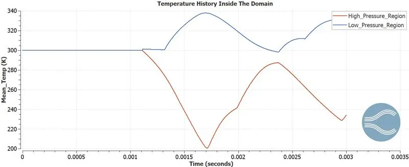
*As the shock wave progresses in to the low pressure region,after some distance it faces resistance,this is due to the formation of high pressure region because of gas compression which is evident from temperature animation.
*From the temperature plot,we can see non linear behaviour and abrupt changes in temperature in both regions,further indicating formation of shock inside the tube.
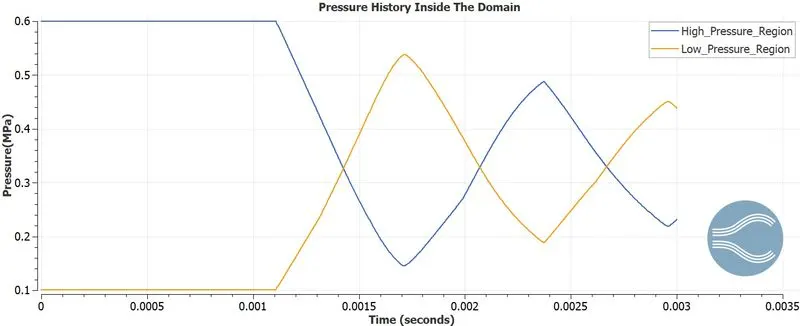
*Also from the pressure animation we can see at the start of event travelling of shock wave into the low pressure region increases pressure in that region ,while pressure decreases behind the wave.The front pressure increase causes shock wave to reflect back and move into other direction.
*From the pressure plot it is evedent that pressure between region varies in a harmonic way,and eventually indicating to settles down to a constant value.
6] CONCLUSION :
*Pressure varies in a harmonic way and reaches steady state.
*Velocity of high pressure species N2 increases suddenly at the initiation of the event or shock.
*Temperature of the species also varies non linearly.
*The behaviour of shock inside a shock tube due to the rupture of diaphragm has been successfully simmulated.