Week 3.5 - Deriving 4th order approximation of a 2nd order derivative using Taylor Table method

Objective - To derive 4th order approximation of a 2nd order derivative using Taylor Table method

Answer -

According to problem statement first we have to derive following schemes for 2nd order derivative -

1. Central difference

2. Skewed right-sided difference

3. Skewed left-sided difference.

1. Central difference -

In this scheme we take information from both sides of a point,at which we want to approximate.
Now to create a taylor table for central scheme,we first have to deside the number of nodes in the stencil,

Number of nodes in the stencil (N) = The order of accuracy (P) + Order of the derivative (Q) - 1

N = 4 + 2 - 1
N = 5

4th order approximation of 2nd order derivative by central difference scheme,

(∂^2f)/(∂x^2) = [af(i-2) + bf(i-1) + cf(i) + df(i+1) + ef(i+2)]/dx^2

Taylor series terms ------->

Stencil ↓	f(x)	Δxf'(x)	Δx^2f''(x)	Δx^3 f'''(x)	Δx^4 f''''(x)
a f(i-2)	a	-2a	4a/2	-4a/3	2a/3
b f(i-1)	b	-b	b/2	-b/6	b/24
c f(i)	c	0	0	0	0
d f(i+1)	d	d	d/2	d/6	d/24
e f(i+2)	e	2e	4e/2	8e/6	16e/24
	0	0	1	0	0

Taylor table for central differencing of 4th order approximation

Writing co-efficients in matrix form,

`[[1, 1, 1, 1, 1],[-2, -1, 0, 1, 2],[4/2, 1/2, 0, 1/2, 4/2],[-8/6, -1/6, 0, 1/6, 8/6],[16/24, 1/24, 0, 1/24, 16/24]]][[a],[b],[c],[d],[e]]=[[0],[0],[1],[0],[0]]`

Calculating the values of co-efficients using matlab inverse matrix function,

>> A=[1 1 1 1 1;-2 -1 0 1 2;2 1/2 0 1/2 4/2;-8/6 -1/6 0 1/6 8/6;16/24 1/24 0 1/24 16/24];
B= [0;0;1;0;0];
>> C=inv(A)*B

C =

   -0.0833
    1.3333
   -2.5000
    1.3333
   -0.0833

Therefore, a = -0.0833 d = 1.3333

b = 1.3333 e = -0.0833

c = -2.5000

2. Skewed right-sided difference

In this scheme we take information from only right side of a point,at which we want to approximate.
Now to create a taylor table for skewed right scheme,we first have to deside the number of nodes in the stencil,

Number of nodes in the stencil (N) = The order of accuracy (P) + Order of the derivative (Q)

N = 4 + 2
N = 6

4th order approximation of 2nd order derivative by skewed right sided scheme,

(∂^2f)/(∂x^2) = [ af(i) + bf(i+1) + cf(i+2) + df(i+3) + ef(i+4) + ff(i+5)]/dx^2

Taylor series terms ------->

Stencil ↓	f(x)	Δxf'(x)	Δx^2f''(x)	Δx^3 f'''(x)	Δx^4 f''''(x)	Δx^5f'''''(x)
a f(i)	a	0	0	0	0	0
b f(i+1)	b	b	b/2	b/6	b/24	b/120
c f(i+2)	c	2c	4c/2	8c/6	16c/24	32c/120
d f(i+3)	d	3d	9d/2	27d/6	81d/24	243d/120
e f(i+4)	e	4e	16e/2	64e/6	256e/24	1024e/120
f f(i+5)	f	5f	25f/2	125f/6	625f/24	3125f/120
	0	0	1	0	0	0

Taylor table for skewed right sided differencing of 4th order approximation

Writing co-efficients in matrix form,

`[[1, 1, 1, 1, 1, 1],[0, 1, 2, 3, 4, 5],[0, 1/2, 4/2, 9/2, 16/2, 25/2],[0, 1/6, 8/6, 27/6, 64/6, 125/6],[0, 1/24, 16/24, 81/24, 256/24, 625/24],[0, 1/120, 32/120, 243/120, 1024/120, 3125/120]][[a],[b],[c],[d],[e],[f]]=[[0],[0],[1],[0],[0],[0]]`

Calculating the values of co-efficients using matlab inverse matrix function,

 A = [1 1 1 1 1 1 ;-5 -4 -3 -2 -1 0;25/2 16/2 9/2 4/2 1/2 0;-125/6 -64/6 -27/6 -8/6 -1/6 0;625/24 256/24 81/24 16/24 1/24 0;-3125/120 -1024/120 -243/120 -32/120 -1/120 0];
B = [0;0;1;0;0;0];
C = inv(A)*B

C =

   -0.8333
    5.0833
  -13.0000
   17.8333
  -12.8333
    3.7500

Therefore, a = -0.8333 d = 17.8333

b = 5.0833 e = -12.8333

c = -13.0000 f = 3.75

3. Skewed left-sided difference.

In this scheme we take information from only left side of a point,at which we want to approximate.
Now to create a taylor table for skewed left scheme,we first have to deside the number of nodes in the stencil,

Number of nodes in the stencil (N) = The order of accuracy (P) + Order of the derivative (Q)

N = 4 + 2
N = 6

4th order approximation of 2nd order derivative by skewed left sided scheme,

(∂^2f)/(∂x^2) = [af(i-5) + bf(i-4) + cf(i-3) + df(i-2) + ef(i-1) + ff(i)]/dx^2

Taylor series terms ------->

Stencil ↓	f(x)	Δxf'(x)	Δx^2f''(x)	Δx^3 f'''(x)	Δx^4 f''''(x)	Δx^5f'''''(x)
a f(i-5)	a	-5a	25a/2	-125a/6	625a/24	-3125a/120
b f(i-4)	b	-4b	16b/2	-64b/6	256b/24	-1024b/120
c f(i-3)	c	-3c	9c/2	-27c/6	81c/24	-243c/120
d f(i-2)	d	-2d	4d/2	-8d/6	16d/24	-32d/120
e f(i-1)	e	-e	e/2	-e/6	e/24	-e/120
f f(i)	f	0	0	0	0	0
	0	0	1	0	0	0

Taylor table for skewed left sided differencing of 4th order approximation

Writing co-efficients in matrix form,

`[[1, 1, 1, 1, 1, 1],[-5, -4, -3, -2, -1, 0],[25/2, 16/2, 9/2, 94/2, 1/2, 0],[-125/6, -64/6, -27/6, -8/6, -1/6, 0],[625/24, 256/24, 81/24, 16/24, 1/24, 0],[-3125/120, -1024/120, -243/120, -32/120, -1/120, 0]][[a],[b],[c],[d],[e],[f]]=[[0],[0],[1],[0],[0],[0]]`

Calculating the values of co-efficients using matlab inverse matrix function,

>> A = [1 1 1 1 1 1 ;-5 -4 -3 -2 -1 0;25/2 16/2 9/2 4/2 1/2 0;-125/6 -64/6 -27/6 -8/6 -1/6 0;625/24 256/24 81/24 16/24 1/24 0;-3125/120 -1024/120 -243/120 -32/120 -1/120 0];
B = [0;0;1;0;0;0];
C = inv(A)*B

C =

   -0.8333
    5.0833
  -13.0000
   17.8333
  -12.8333
    3.7500

Therefore, a = -0.8333 d = 17.8333

b = 5.0833 e = -12.8333

c = -13.0000 f = 3.7500

Now we have to write code in MATLAB to compare analytical derivative of a function ,'exp(x)*cos(x) ,with above 3 numerical approximations and have to compare error between abhove schemes.

Code Explaination -

First I created a function named as [central_error,right_skewed_error,left_skewed_error]= taylor_table(x,dx).And I computed error related to each scheme inside a single function,instead of creating separate function to compute error for each scheme,and also calculated the second order analytical derivative of the given function.

Second order analytical derivative -

= `e^xcosx`

= `e^x(-sinx)+cosx e^x`

First derivative = `e^x(cosx-sinx)`

= `e^x(-sinx-cosx)+(cosx-sinx)e^x`

Second derivative = `-2e^xsinx`

function [central_error,right_skewed_error,left_skewed_error]= taylor_table(x,dx)
%coefficient values for central differencing,right skewed diferencing,left skewed differencing 
a = -0.0833;  a2 = -0.8333;
b =  1.3333;  b2 =  5.0833;
c = -2.5000;  c2 = -13.0000;
d =  1.3333;  d2 =  17.8333;
e = -0.0833;  e2 = -12.8333;
              f2 =  3.7500;
% Numerical approximation using central,right skewed and left skewed
% differencing
central_differencing = ((a*exp(x-2*dx)*cos(x-2*dx))+(b*exp(x-dx)*cos(x-dx))+(c*exp(x)*cos(x))+(d*exp(x+dx)*cos(x+dx))+(e*exp(x+2*dx)*cos(x+2*dx)))/(dx^2);
right_skewed =((a2*exp(x+5*dx)*cos(x+5*dx))+(b2*exp(x+4*dx)*cos(x+4*dx))+(c2*exp(x+3*dx)*cos(x+3*dx))+(d2*exp(x+2*dx)*cos(x+2*dx))+(e2*exp(x+dx)*cos(x+dx))+ (f2*exp(x)*cos(x)))/(dx^2);
left_skewed = ((a2*exp(x-5*dx)*cos(x-5*dx))+(b2*exp(x-4*dx)*cos(x-4*dx))+(c2*exp(x-3*dx)*cos(x-3*dx))+(d2*exp(x-2*dx)*cos(x-2*dx))+(e2*exp(x-dx)*cos(x-dx))+ (f2*exp(x)*cos(x)))/(dx^2);
%Computing error
analytical_value = -2*exp(x)*sin(x);
central_error = abs(central_differencing - analytical_value);
right_skewed_error = abs(right_skewed-analytical_value);
left_skewed_error = abs(left_skewed -analytical_value);
end

After this in the main code I created the for loop,for the range of dx.And inside the for loop I call out the function,which calculated the error for each scheme for i'th index of dx.

clear all
close all
clc
% Inputs
x = pi/3; dx = linspace(pi/4,pi/4000,20);

%Computing error for range of dx

for i = 1:length(dx)
    [central_error(i),right_skewed_error(i),left_skewed_error(i)]= taylor_table(x,dx(i));
end
% Plot for compairing all 3 errors with range of dx
loglog(dx,central_error,'r')
hold on
loglog(dx,right_skewed_error,'g')
loglog(dx,left_skewed_error,'b')
xlabel('range of dx')
ylabel('error')
legend('central error','right skewed error','left skewed error')

Then I plotted the graph compairing the error by each scheme over the range of dx.

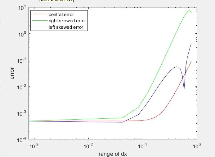
From the plot we can see that central difference has the smallest error,compared to skewed left sided scheme and skewed right sided scheme.Therefore,

central differencing error < skewed left sided error < skewed right sided error

Why skewed scheme is useful and what skewed scheme can do that central differencing scheme can't ?

Central difference scheme requires information from both side of the data point ,which is useful in diffusion problems.But when we are dealing with bounday condition ,where we have only one direction to go,in that case skewed scheme is useful,since it requires data from one side only,since central scheme requires data from both side it's not useful at boundary problem.