Week 5: Prandtl Meyer Shock problem
Aim:
* To simulate the Prandtl Meyer expansion shock and investigate the effect of SGS parameters on shock location and
temperature.
Objective :
*Describe what boundary conditions are typically used foe shock flow problems.
*Describe physics behind shock waves.
*Discuss the effect of SGS parameter on shock location and cell count value.
*Show the mesh generation using paraview.
Introduction and Theory :
* At the molecular level fluid particles travel in a continuam,when an obstruction is suddenly introduced in the flow,something interesting happens.The particle in front of it slow down instantaniously creating an increase in local pressure.Since the fluid is continuam the information of whatever happens in one place is transmitted to other regions in the form of pressure waves.This pressure wave then causes the oncoming fluid to adjust it's properties.
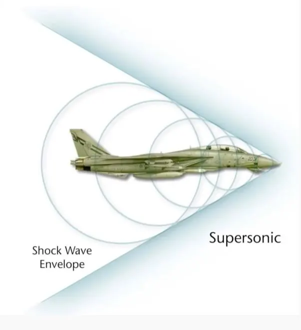
* Now we know that, sound travel through the medium in the form of comression and rarefaction.But the information propagation in fluid happens through the accoustics waves which travels at the speed of sound.
* When the fluid particles are travelling faster than the speed of sound,and since the information transfer can not happen faster than the speed of sound,the oncoming particles don't have any information about the coming obstruction in front until they actually reach it.The moment they reach it,the extreme collsion of particles with themselves and with the object occurs,which manifest itself as a shockwave.
Mach Number -
* Mach number is a dimensionless number which is very important while studing the shocks. Mach number is the ratio of velocity of the fluid(`mu`) to the velocity of sound in that medium(a).So clearly if mach number is greater than 1,this means fluid is travelling faster than the speed of sound meaning,there is no time for the information to propagate,these flows are called as supersonic flows.
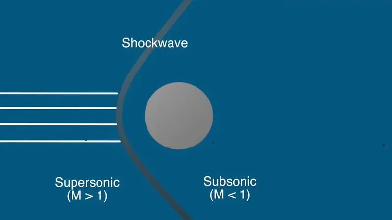
* A moving shock is called as shock wave which is very thin in the order of 200 nanometers and it's under this region where
fluid undergoes sudden change of properties.The mach number decreases across the shockwave,along with sudden rise in pressure, density and temperature.Shockwave is also a irreversible process because of the extreme reactions produced by the collision of the particles.
* In some aerospace apllications an engineer always tries to reduce the shock as,it causes vibrations and increase in drag.
Even in commercial aircraft which never goes supersonic,there are regions over the wing where,flow can locally go supersonic, this is the exact region why commercial airplanes have swept back wings.When air now flows over the wing,it sees a thinner wing because only a component of the velociy is perpendicular to it and doesn't accelerate to supersonic speeds.
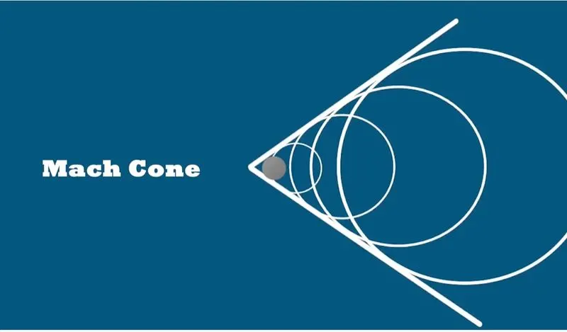
* When a stationary object emmits sound waves at a certain frequency,the waves are genearllyspherical in nature and travel at the speed of sound.The moment an object starts moving,the sound waves in front of it compressed increasing the apparant frequency and the ones behind elongate decrasing the apparant frequency,this effect is known as doppler effect .When the object travels faster than the speed of sound,the sound waves that are emitted form a cone known as the Mach cone.
Types of Shock Waves -
Bow or Detached Shock Wave -
* This type forms in front of the ball is known as bow shock or detached shock.It is special that it does not connected to the
ball in anyway.It is also very complicated to study,since it very much depends on the geometry of the object.BUt in general
bow shocks will form only with blunt objects .
Oblique Shock Wave -
* Now as the object becomes more streamlined,eventually more pointed the shock wave will too,until it hits a critical point,where bow shock becomes an attached oblique shock.The crititical point depends on the speed of the flow and the angle of the cone. Aircraft designers wants to avoide bow shocks at all costs,since they provide detrimental amount of drag.Oblique shocks are formed when,the supersonic flow is rapidly redirected on to itself.This flow has little effect on drag
because they don't actually slow down the air,they actually speed it up.
Normal Shock Wave -
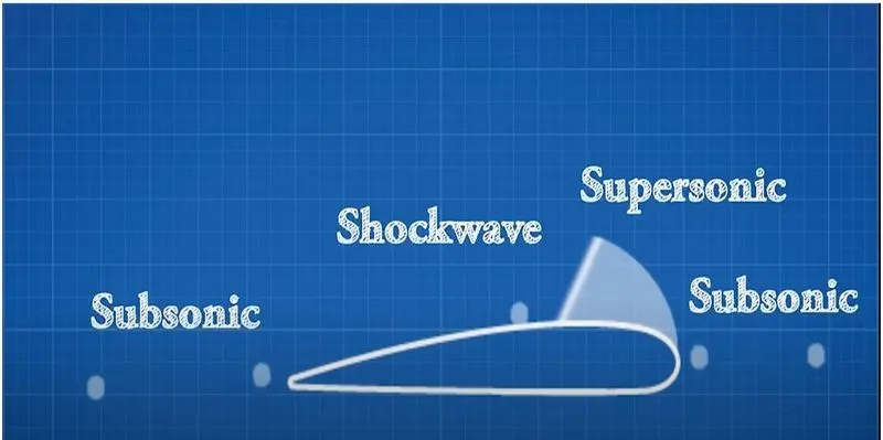
* When the flow is not turned at all,the resulting shock is called as normal shock since it forms perpendicular to the surface.
Normal shocks occur when there is change in the flow area and similar to bow shocks they change the flow from supersonic
to subsonic and simillar to oblique shocks they are also attached to the body.
Normal shocks often forms on the upper surface of the wing,because the flow speeds up enough locally to go supersonic. Since normal shocks also have drag,high speed aircrafts often have swept wings so these normal shocks behave like oblique shocks and airspeed is maintained.
Expansion Waves -
* Expansion shocks are formed when,the supersonic flow suddenly turns around the corner as shown in figure.It is opposite of oblique waves,where waves are turned onto themselves,whereas in this waves are turned away from themselves. These waves are also known as prandtl meyer expansion fan which is made up of infinite amount of oblique waves.
WHY WE NEED INITIAL CONDITIONS AND BOUNDARY CONDITIONS ?
* Consider a example of a pipe whose one end is placed at a heating source i.e. heat is continuously being added at one end.
now if we want to know the temperature distribution along the pipe and want to find the scalar temperature field in space and time ,we need initial and boundary conditions to solve the respective P.D.E.
TYPES OF BOUNDARY CONDITIONS -
There are 5 types ofnboundary conditions -
1. Dirichlet boundary condition
2. Neumann boundary condition
3. Robin's boundary condition
4. Mixed boundary condition
5. Cauchy boundary condition
1. Dirichlet boundary condition
* This condition specifies the value that the unknown function needs to take on along the boundary of the domain.i.e.solution of the differential equation takes the value at perticular boundary points.
2. Neumann boundary condition
* This specifies the values that the derivative of the solution is going to take in the direction normal to the boundary of the domain.
3. Robin's boundary condition
* This is a weighted combination of Dirichlet boundary condition and Neumann boundary condition in all the parts of the boundary.
4. Mixed boundary condition
* Mixed boundary condition refer to yhe case in which Dirichlet boundary conditions are prescribed in some parts of the boundary while Neumann boundary conditions exists in other.
5. Cauchy boundary condition
* This boundary condition specifies both the functional value and normal derivative on the boundary of the domain.
It differs from Robin's boundary condition because the Cauchy condition implies the imposition of two constraints(one Dirichlet boundary condition and + one Neumann boundary condition),the Robin's boundary condition implies only one constraint on the linear combination of the unknown function and it's derivative. Here the conditions are defined at the same location.This is the main difference between Robin's boundary condition and
Cauchy boundary condition
Boundary conditions Used for shock flow problems -
* For copressible flows,the inlet conditions are generally known hence,constant value is given at the domain i.e Dirichlet
boundary condition. In shock flow problems outlet conditions are not known because,shock causes huge variation in flow properties,which leads to gradient across the normal surface.This can be extrapolated from the inlet conditions and the basic properties of the flow by defining the zero normal gradient i.e. Neumann boundary condition at the outlet.
4] Solution Procedure :
To simulate steady state flow over a throttle body ,we will follow the below procedure :-
Geometry Creation --> Case Setup --> Solution --> Post Processing
4.1] Geometry Creation :
* Launch Converge and start a new project.
* Drag and drop the .stl model in converge.
* In converge ,geometries are represented as triangles.So we need to group these triangles to create boundaries.This is the
fundamental step in Converge.
Geometery => Boundary => Flag => click on add and add 3 boundaries => rename first boundary as inlet => using by angle triangle selection,select front face triangles => apply.
* Simillarly flag outlet,top,bottom,font and back.
* As our flow is internal,we want all the normals to point into the fluid domain.To do that,
click on normal toggle => transform => normal => click on triangle with outside pointing normal => apply
* Make sure that geometry is clean,
Diagnosis => find => no errors.
4.2] Case Setup :
* Click on Begin Case Setup => General Flow => Done.
*Our working fluid will be air .
*Materials => Predefined mixture => Air => uncheck reaction mechanism => check species => Apply & Done.
*Keep default global transport parameters.
*In species add oxygen and nitrogen.
*We will be running steady state simulation.To set this follow below steps,
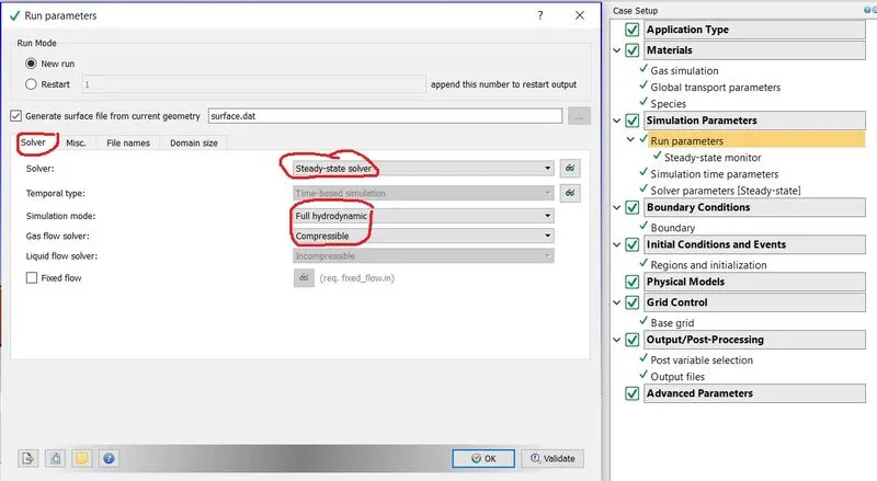
*a] Run Parameters => Solver => select solver type steady state solver => simulation mode full hydrodynamic => Gas flow solver compressible.
b] In Misc => check steady state monitor => uncheck use shared memory.
*In converge it is mandatory in steady state simulation to define monitor points,so that solver know when to terminate the
simulation in order to save computation time.
*Steady State Moniter => Add Config. => then add average velocity,total pressure , mass flow rate.
*We need to define the minimum number of cycles we want simulation to run before terminating, set it to 500 cycles.
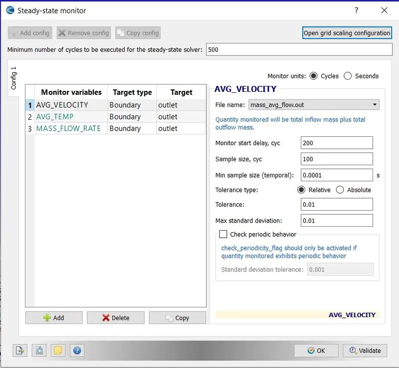
*Also we don't want the solver to moniter the points from the start of the simulation,as we know simulation will be
unsteady at the start of the simulation.Hence we will moniter the solution after 200 cycles and our sample size will be 100.
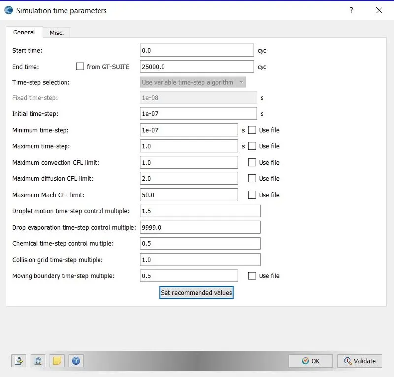
*Simulation time parameters =>
Start Time - 0 cycles
End Time - 25000 cycles
Initial Time Step - 1e-7 sec.
Minimum Time Step - 1e-7 sec.
Maximum time step - 1 sec.
Maximum Convection CFL limit - 1.0.
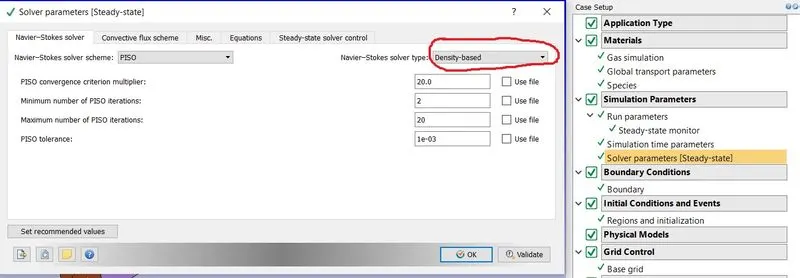
*Solver Parameters =>
Navier-Stokes solver Scheme => PISO
Navier-Stokes solver Type => Density Based
Pressure Preconditioner - none
Maximum convection CFL limit(Final Stage) - 0.5
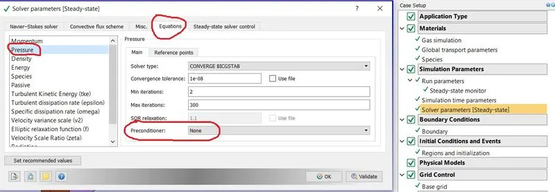
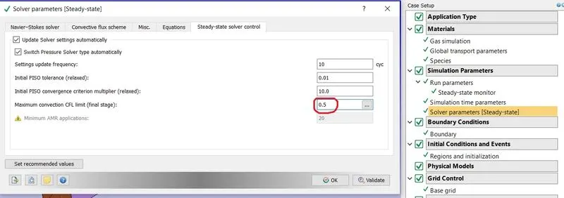
*Now before setting the boundaries,set initial region and set initial pressure and define air species.This region will be assigned to each boundary.
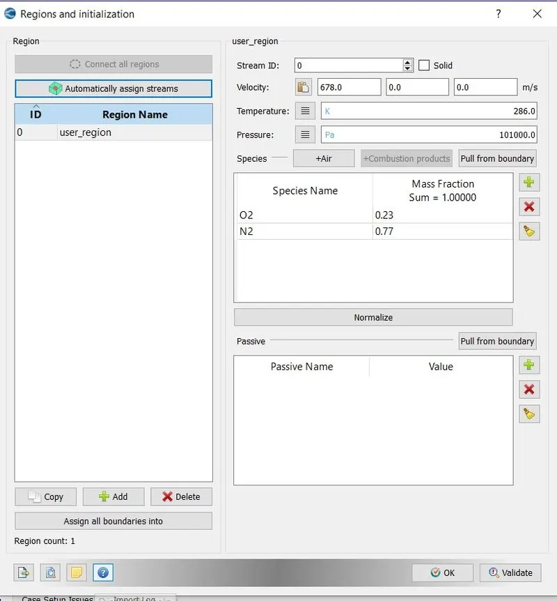
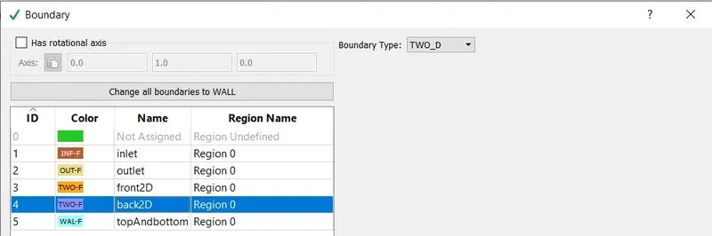
*Boundaries =>
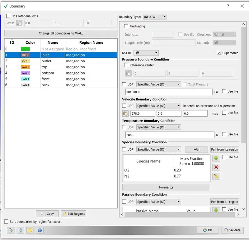
Inlet -
Boundary Type - INFLOW
Pressure Boundary Condition - Specied value - 101000 Pa
Temperature Boundary Condition - Specied value - 286 K
Species Boundary Condition - select Air
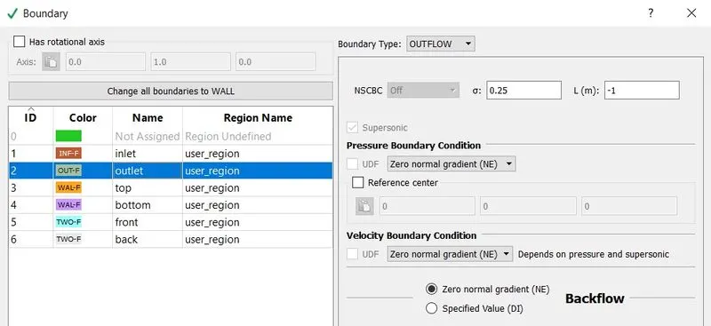
Outlet -
Boundary Type - OUTFLOW
Pressure Boundary Condition - Zero normal gradient(NE)
Velocity Boundary Condition - Zero normal gradient(NE)
Backflow -Zero normal gradient(NE)
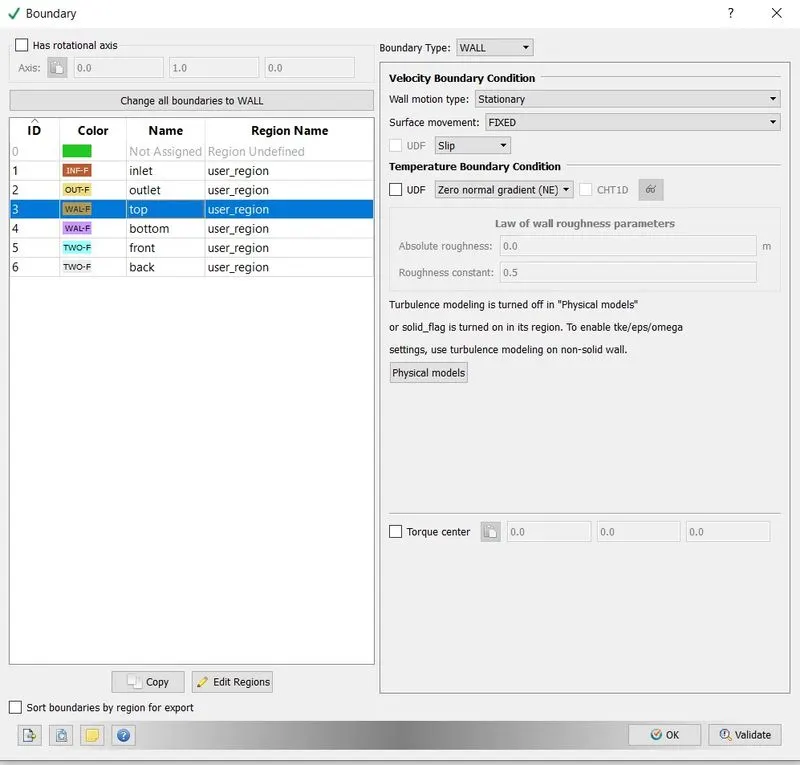
top
Boundary Type - Wall(slip)
Temperatue Boundary Condition - Zero normal gradient(NE)
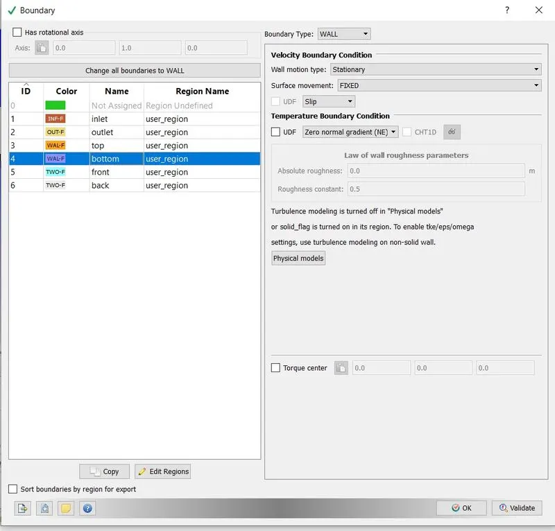
bottom
Boundary Type - Wall(slip)
Temperatue Boundary Condition - Zero normal gradient(NE)
Front -
Boundary Type - TWO_D
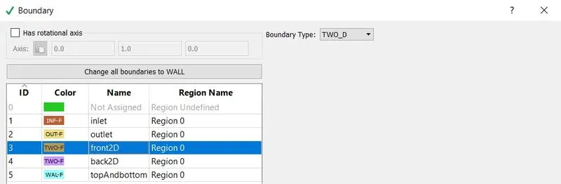
Back -
Boundary Type - TWO_D
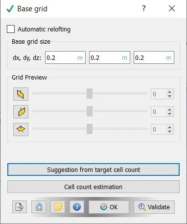
*In converge mesh generation is a fully automatic process.Converge uses cut cell method to generate the mesh.
Base Grid = dx= 0.2 ; dy = 0.2 ; dz = 0.2 => ok
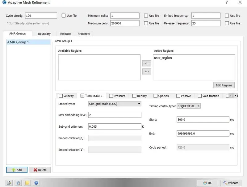
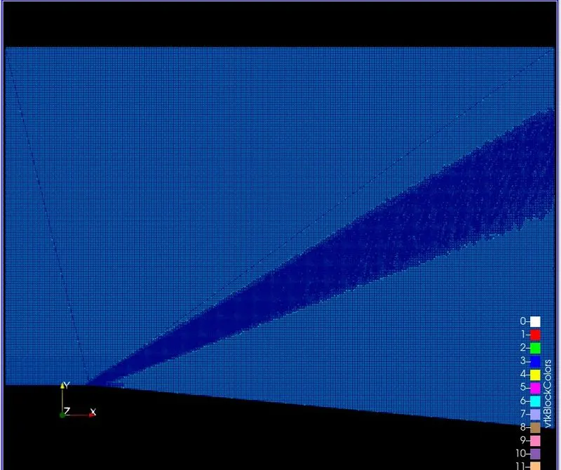
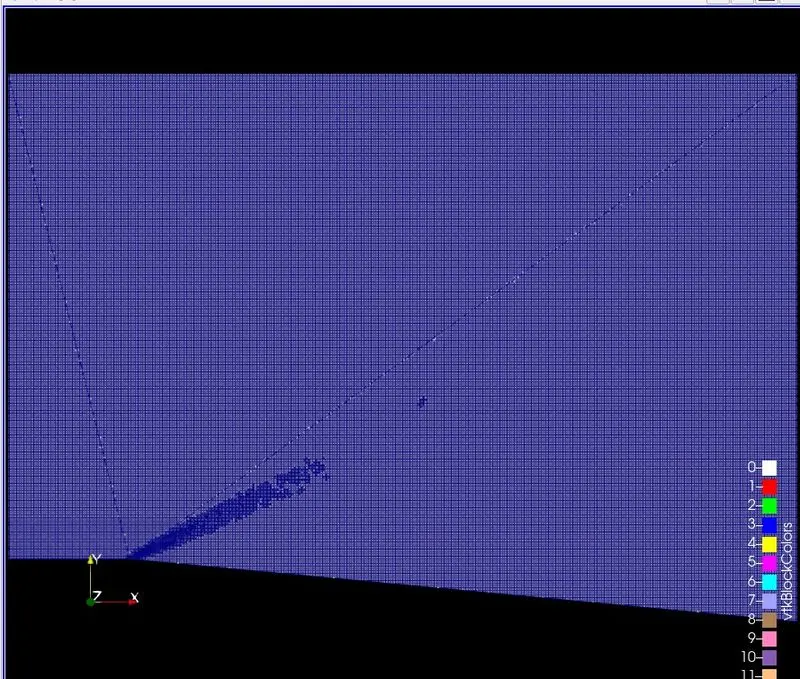
*Now we want to moniter how the flow properties changes as the shock forms.We will moniter temperature deviation in the flow.For that we will do the adaptive mesh refinement based on temperature deviation.We need to provide sub grid criterion.So whenever subgrid scale temperature difference is greater than user specified value our mesh will refine.
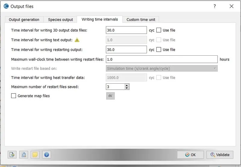
*In post variable selection,select the variables which needs to be post processed and set species mass fraction.
*We want our post processed graphes and animations to be smooth,so we want ample amount of ouput files.It is good practice to have at least 100 3D output files and same amount of text output files.
Solution :
*For running the simulation,first we need to export all the input files to the folder where we want to save our output files,
File => Export => Export Input Files => select the desired folder => Export.
*Now we will use CYGWIN command prompt to run our simulation.But before running the simulation first we need executables which willl solve the simulation,for that paste mpiexec.exe and converge.exe into the folder where we have exported all our input files.
*Now using CYGWIN command prompt,navigate to the folder where all the input files are exported,and type the below command,
mpiexec.exe -n 4 converge.exe restricted </dev/null> logfile &
*In the above command ,mpiexec.exe will help us to run our simulation in parallel,-n 4 are the number of cores on which we
want to run our simulation.As we are using the version of converge which has limit on the size of the file it can solve hence the command restricted.And the last part of the command dump all the data that is being generated into the logfile, which we can access during simulation procedure to see where our simulation has reached.
*The above command will create a folder named output containing all the generated 3D output data.As we will be using paraview as the postprocessing tool.Hence we need to convert these output files into the format that paraview can read.For this we will use converge post convert tool.
Go to converge post processing 3D =>give case name => select the file type => navigate to the output folder and select it
=> select all files => select all variables => convert.
This will create group file ,which will be used by paraview to post process our results.
Post Processing :
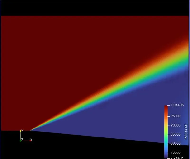
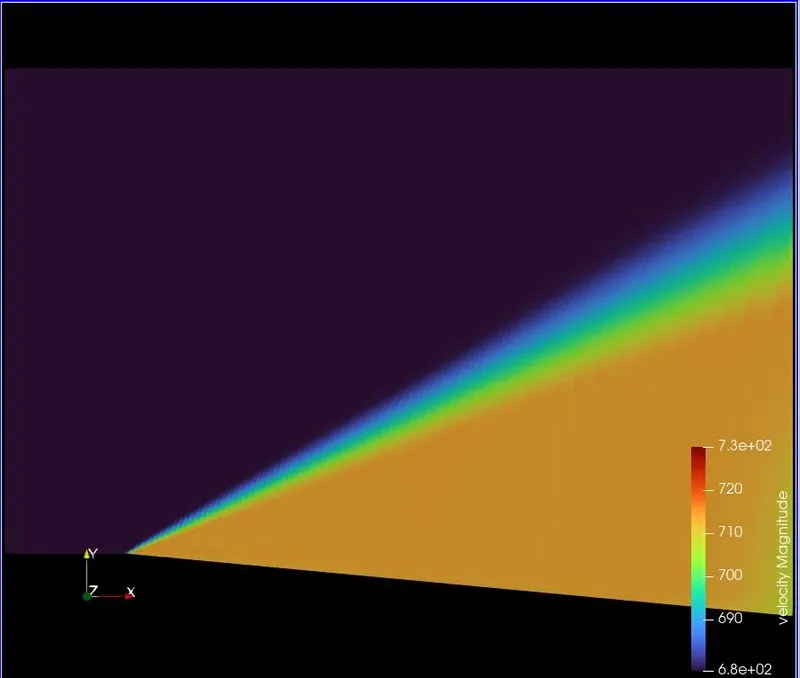
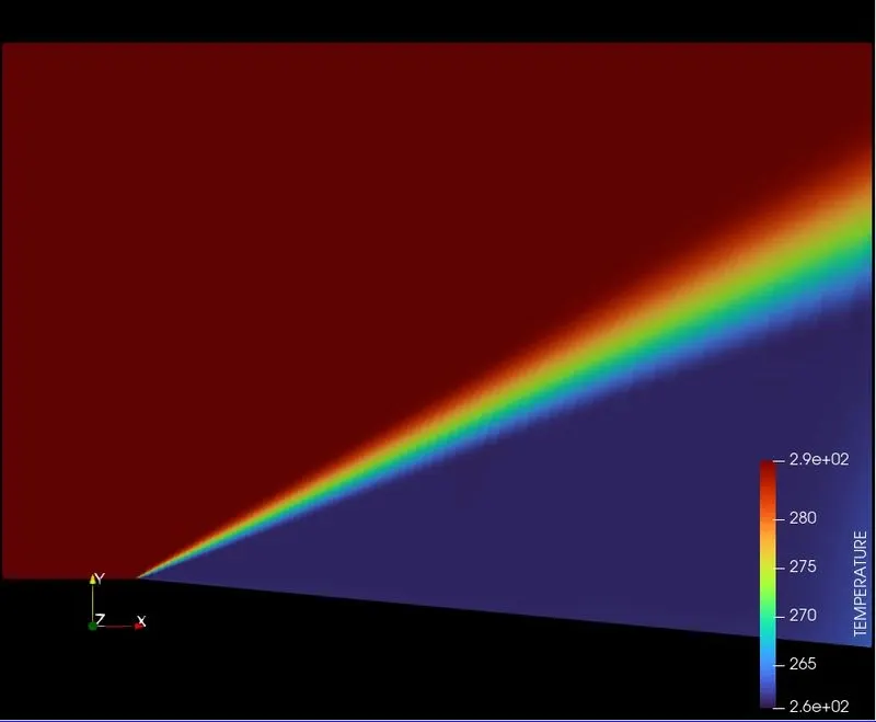
Case 1(Sub Grid Scale 0.005) =>
Pressure Contour -
Velocity Contour-
Temperature Contour -
Mesh -
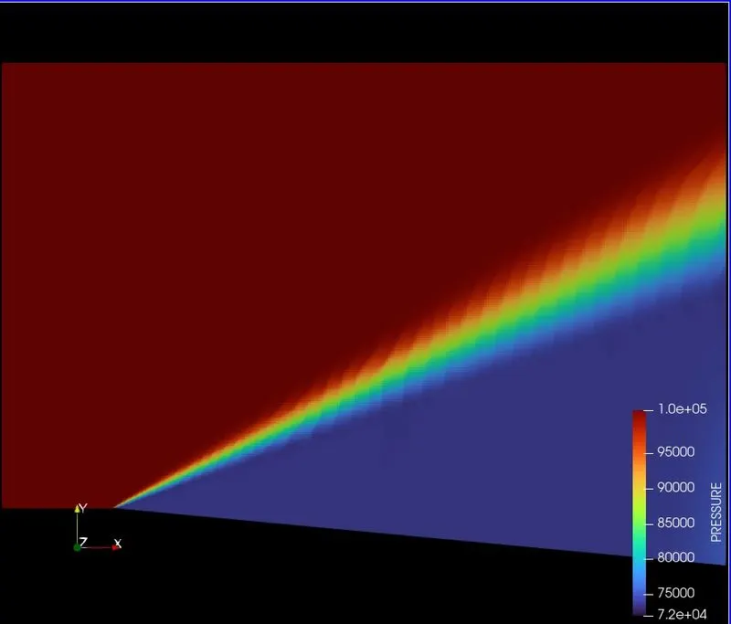
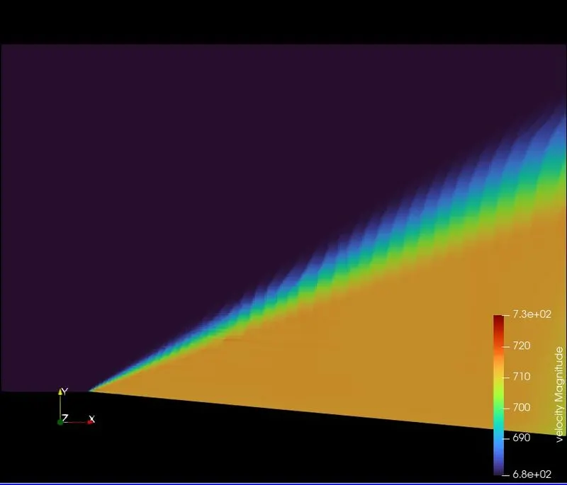
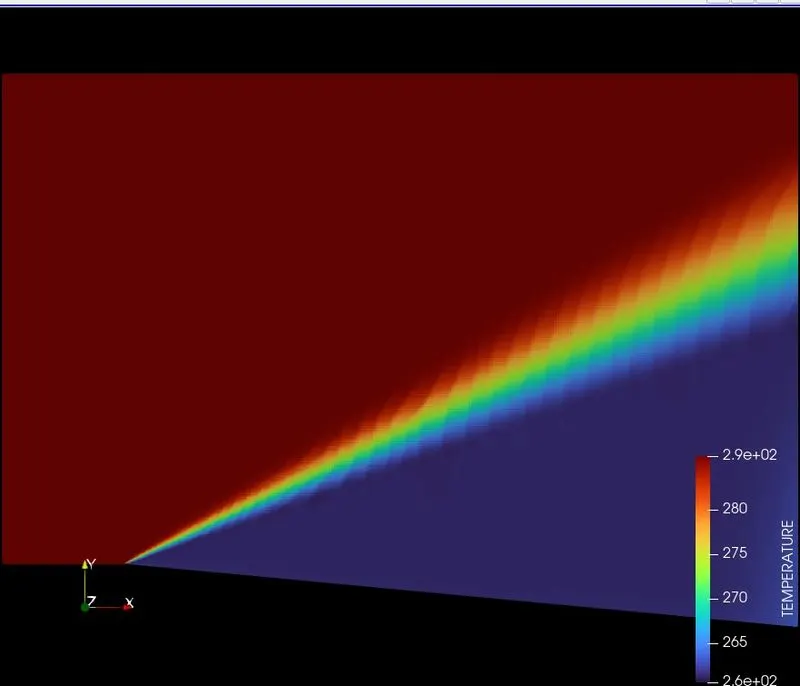
Case 2 (Sub Grid Scale 0.05)=>
Pressure Contour -
Velocity Contour -
Temperature Contour -
Mesh -
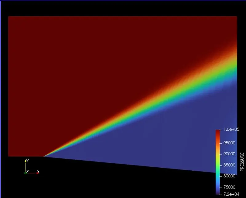
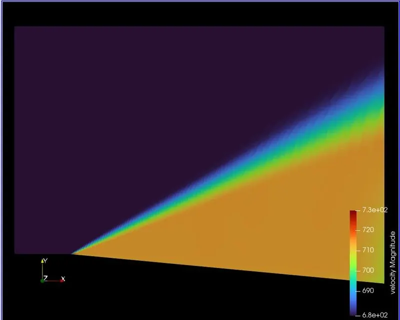
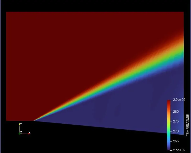
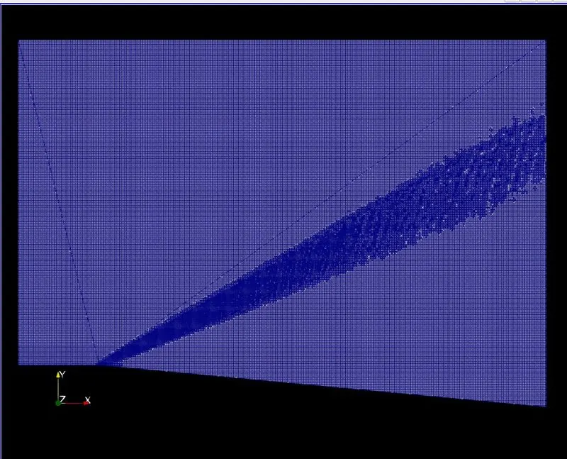
Case 3 (Sub Grid Scale 0.01) =>
Pressure Contour -
Velocity Contour -
Temperature Contour -
Mesh -
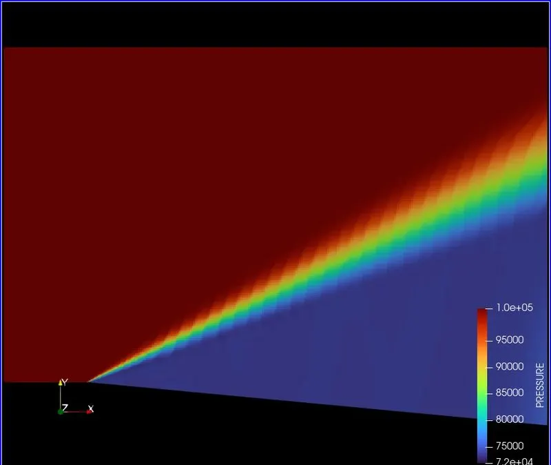
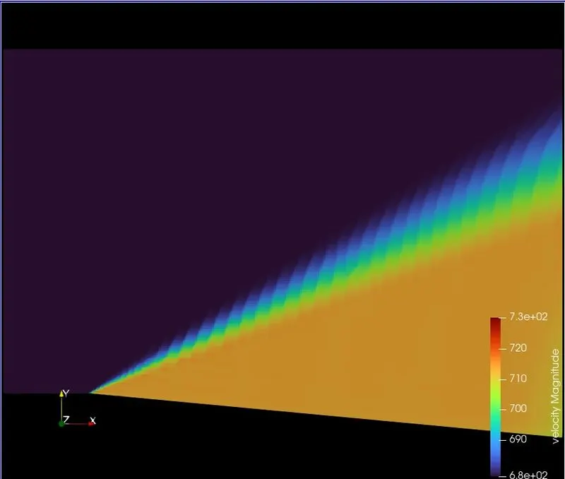
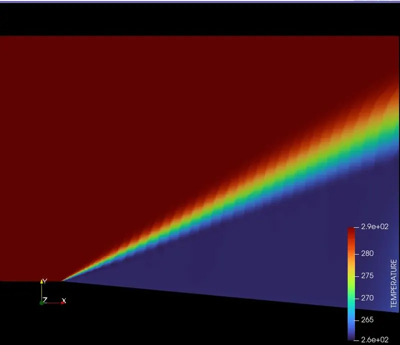
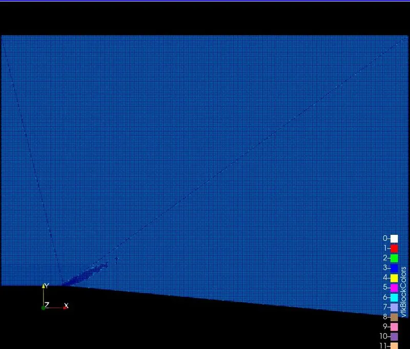
Case 4 (Sub Grid Scale 0.1)=>
Pressure Contour -
Velocity Contour -
Temperature Contour -
Mesh -
Plots :
Animations :
Case 1(SGS - 0.005) -
Velocity - https://www.youtube.com/watch?v=iN9vls8Lb9I
Temperature - https://www.youtube.com/watch?v=JDOY7i5bOx0
Pressure - https://www.youtube.com/watch?v=rO0pmTgHkLo
AMR - https://www.youtube.com/watch?v=0PYbf8n3YzY
https://www.youtube.com/watch?v=Q8QLd-YP9jo
Case 2(SGS - 0.05) -
Velocity - https://www.youtube.com/watch?v=qzvRHQkLOfk
Temperature - https://www.youtube.com/watch?v=X-qaLYYpTLI
Pressure - https://www.youtube.com/watch?v=L3te4euMDeI
AMR - https://www.youtube.com/watch?v=gRlnMpokz8E
https://www.youtube.com/watch?v=Eht5OhD5XfI
Case 3(SGS - 0.01) -
Velocity - https://www.youtube.com/watch?v=DBnTmOgjfc0
Temperature - https://www.youtube.com/watch?v=ZH7hYqAlvb4
Pressure - https://www.youtube.com/watch?v=u-rjcC5-Vws
AMR - https://www.youtube.com/watch?v=AvsKyJM0jsQ
https://www.youtube.com/watch?v=dJownBHQBe8
Case 4(SGS - 0.1) -
Velocity - https://www.youtube.com/watch?v=if6PEVBNNMI
Temperature - https://www.youtube.com/watch?v=ckDb7uawMgE
Pressure - https://www.youtube.com/watch?v=WQsKP0XDsXc
AMR - https://www.youtube.com/watch?v=56FHzyt_IHA
https://www.youtube.com/watch?v=-etr4cDTB1k
Discussion -
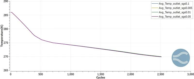
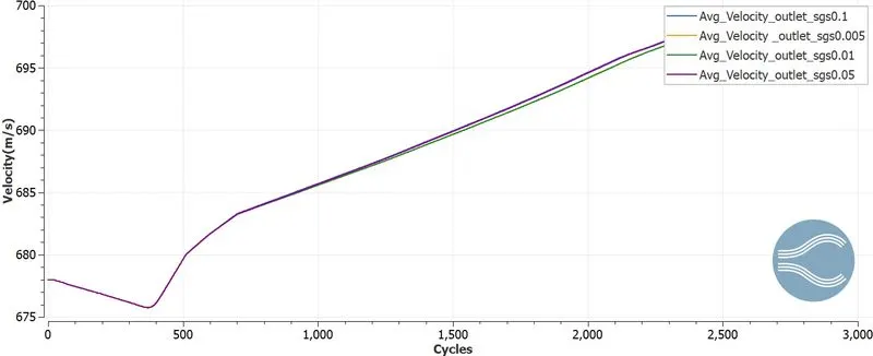
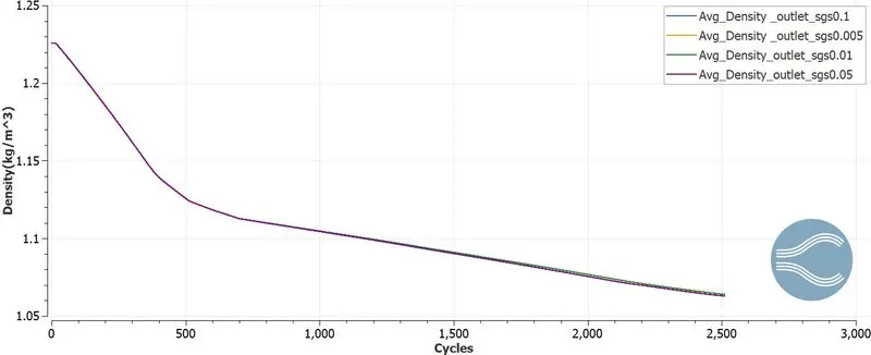
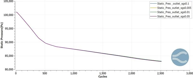
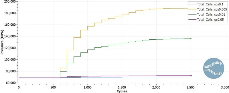
*From the plot of total cells,it is very much obvious as the subgrid scalling is decreased ,cell count is increased.But this does not cause major variation in the final average temperature at the outlet.Same can be said for average velocity and static pressure at the outlet.
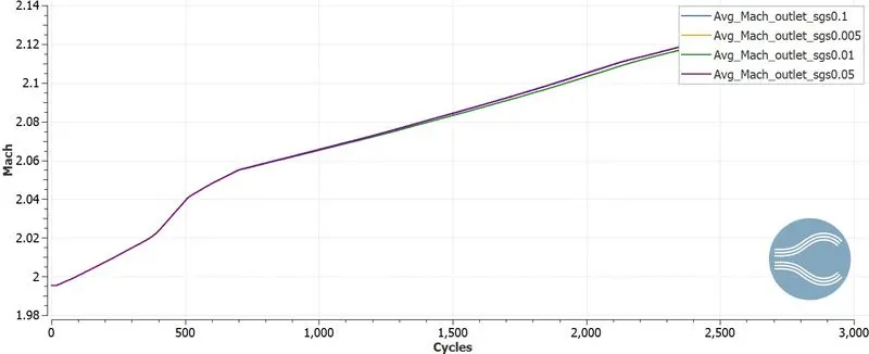
*From the mach number plot,we can see that,the moment it meets the convex corner ,expansion fan formed ,mach number increased ,but then towards outlet it normalises.Since shock flow is an irrevesible process,this will cause increase in entropy.
Validation :
*To validate our results we need to compare analytical and numerical results.We can get the analytical values by doing
following calculation -
`f=sqrt((gamma+1)/(gamma-1))arctansqrt(((gamma-1)/(gamma+1))(M^2-1))-arctansqrt(M^2-1)`
and `f_2=f_1+theta`
*From the John anderson text we got value for `f(2)=26.37 deg` .
Thus,`theta=f(M_2)-f(M_1)` and`f(M_2)=theta +f(M_1)`.
We got `M_2= 2.20`.
For temperature,pressure and density,we will use following formulae ,
`P_2=P_1*[[(1+(gamma-1)/2)*M_1^2]/[(1+(gamma-1)/2)*M_2^2]]^(gamma/(gamma-1))`
`T_2=T_1*[(1+(gamma-1)/2)*M_1^2]/[(1+(gamma-1)/2)*M_2^2`
Given initial conditions :
T = 286 K,`rho=1.23 (kg)/m^3`, P = 1 bar
And from analytical calculations at outlet we got following results,
`T_2'=269.53k`
`P_2=0.729` bar
`rho_2=1.124 (kg)/(m^3)`
Numerical Results
`T_2'=269.53k`
`P_2'=0.82`bar
`rho_2'=1.059 (kg)/m^3`
Thus,
Error Percentage -
Temperature -`(269.53-261.5)/(261.5)*100` = 3 %
Simillarly, Density = 6 %
Pressure = 3%
Conclusion :
*When th esupersonic flow meets a convex corner,it forms an expansion fan leading to a spontaneous change of flow variables such as velocity,temperature,density etc.
*The effect of sgs temperature on cell count increases as sgs temperature value gets low..Due to the increase in cell count with the decrease in sgs ,a more accurate shock location can be obtained.
*Thus in this project we have successfully studied Prandtl Meyer expansion fan.