Week 3: Flow over a backward facing step
1] Aim :
To simulate flow over a backward facing step using converge CFD.
2] Objective :
* Run the simulation for 3 base mesh sizes.
Case 1 - dx = dy = dz = 2e-3 m
Case 2 - dx = dy = dz = 1.5e-3 m
Case 3 - dx = dy = dz = 1e-3 m
*Show images of mesh for each case,also show pressure and velocity contours.
*Show th eplots of velocity,mass flow rate,pressure and total cell count for each case.
*Explain where and why separation is taking place.And create and upload animations.
3] Introduction :
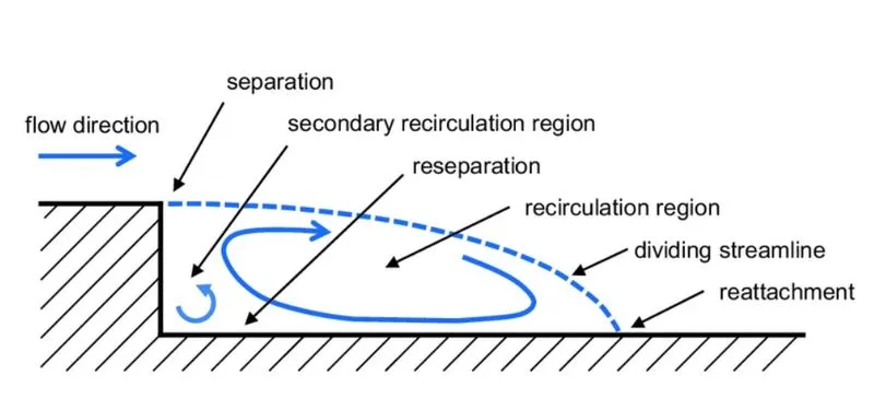
*Consider a 2D laminar,flow over the backward facing step.The geometry of the backward facing step is shown
in the following figure.Consider TWO_D boundary condition on every wall.We will perform a stady state simulation using
Converge by creating 3 different mesh sizes,to observe the effect of mesh size on final results.
*The backward facing step is a standard geometry used for visualizing the recirculationg flow and validating turbulence models.Backward facing step flow is one representative model for separation flows,which is widely used in aerodyanamic flows,condensers,vehicles etc.
4] Solution Procedure :
To simulate backward facing step flow ,we will follow the below procedure :-
Geometry Creation --> Case Setup --> Solution --> Post Processing
4.1] Geometry Creation :
* Launch Converge and start a new project.
*Drag and drop the .stl model in converge.
*In converge ,geometries are represented as triangles.So we need to group these triangles to create boundaries.This is the
fundamental step in Converge.
Geometery => Boundary => Flag => click on add and add 4 boundaries => rename first boundary as inlet => using by angle triangle selection,select front face triangles => apply.
*Simillarly flag outlet,top and bottom, front2D and back2D boundaries.
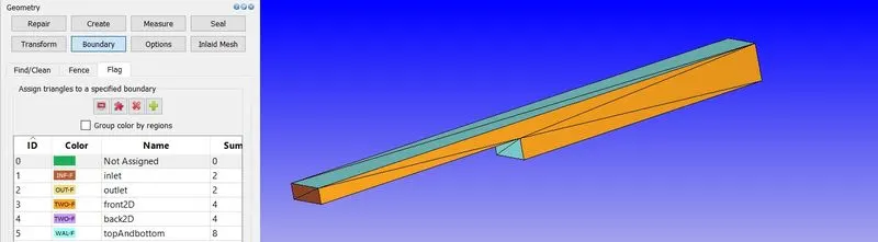
*As our flow is internal,we want all the normals to point into the fluid domain.To do that,
click on normal toggle => transform => normal => click on triangle with outside pointing normal => apply
*Make sure that geometry is clean,
Diagnosis => find => no errors.
4.2] Case Setup :
*Click on Begin Case Setup => General Flow => Done.
*Our working fluid will be air .
*Materials => Predefined mixture => Air => uncheck reaction mechanis => check species => Apply & Done.
*Keep default global transport parameters.
*In species add oxygen and nitrogen.
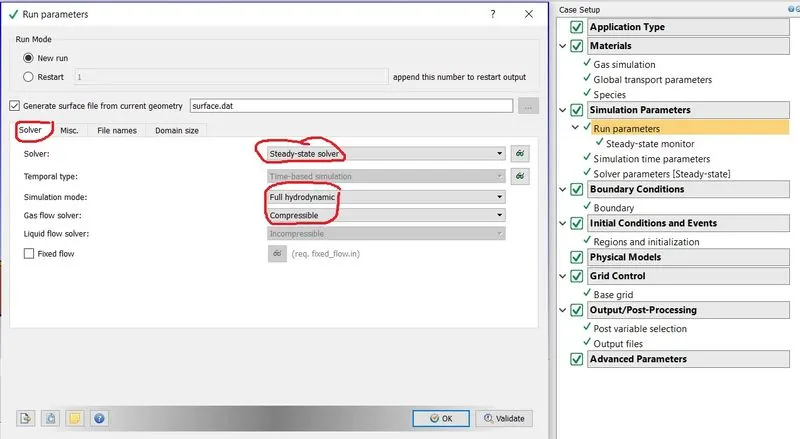
*We will be running steady state simulation.To set this follow below steps,
*a] Run Parameters => Solver => select solver type steady state solver => simulation mode full hydrodynamic => Gas flow solver compressible.
b] In Misc => check steady state monitor => uncheck use shared memory.
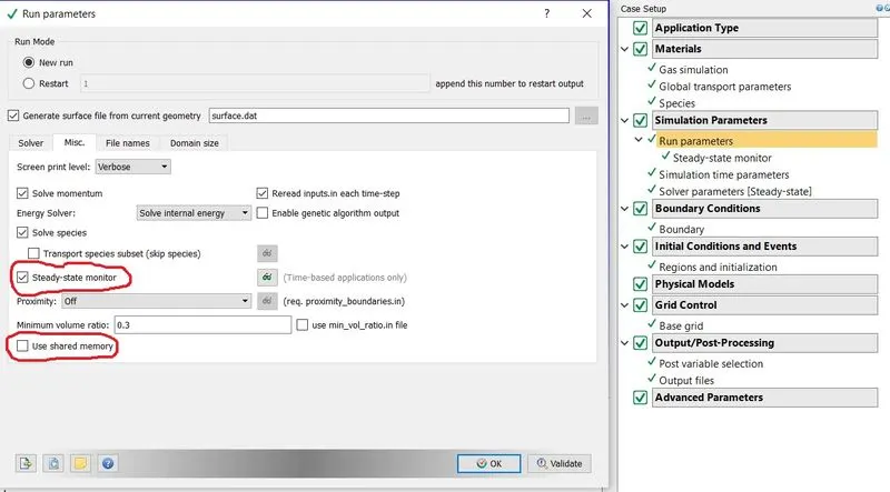
*In converge it is mandatory in steady state simulation to define monitor points,so that solver know when to terminate the
simulation in order to save computation time.
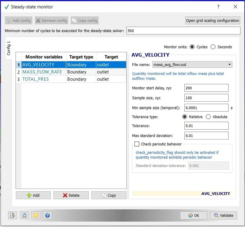
*Steady State Moniter => Add Config. => then add average velocity,total pressure , mass flow rate.
*We need to define the minimum number of cycles we want simulation to run before terminating, set it to 500 cycles.
*Also we don't want the solver to moniter the points from the start of the simulation,as we know simulation will be
unsteady at the start of the simulation.Hence we will moniter the solution after 200 cycles and our sample size will be 100.
*Simulation time parameters =>
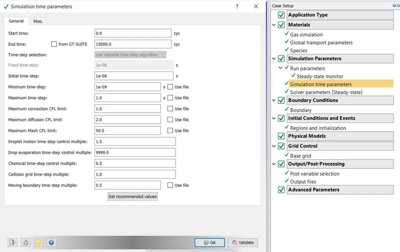
Start Time - 0 cycles
End Time - 15000 cycles
Initial Time Step - 1e-6 sec.
Minimum Time Step - 1e-6 sec.
Maximum time step - 1 sec.
Maximum Convection CFL limit - 1.0.
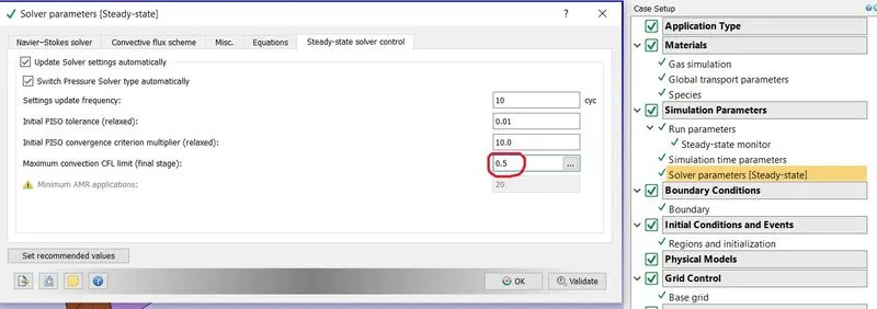
*Solver Parameters =>
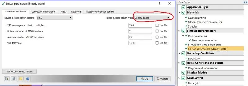
Navier-Stokes solver Scheme => PISO
Navier-Stokes solver Type => Density Based
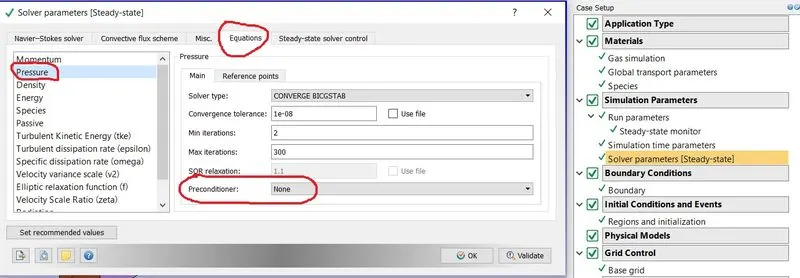
Pressure Preconditioner - none
Maximum convection CFL limit(Final Stage) - 0.5
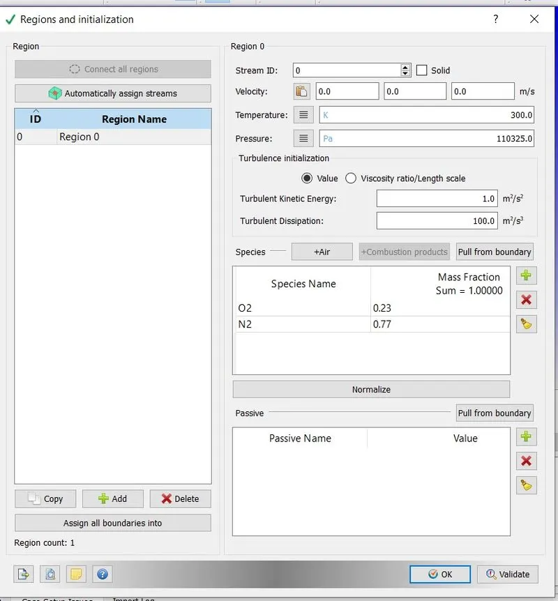
*Now before setting the boundaries,set initial region and set initial pressure and define air species.This region will be
assigned to each boundary.
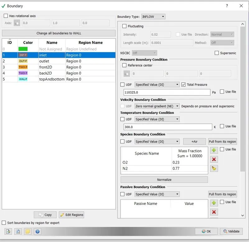
*Boundaries =>
Inlet -
Boundary Type - INFLOW
Pressure Boundary Condition - Specied value - 110325 Pa
Temperature Boundary Condition - Specied value - 300 K
Species Boundary Condition - select Air
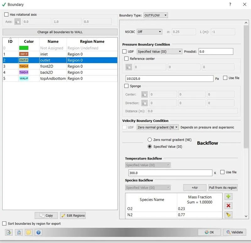
Outlet -
Boundary Type - OUTFLOW
Pressure Boundary Condition - Specied value - 101325 Pa
Temperature Boundary Condition - Specied value - 300 K
Species Boundary Condition - select Air
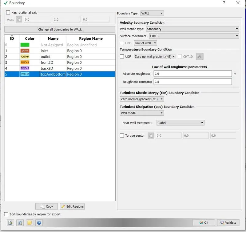
topAndbottom -
Boundary Type - Law of Wall
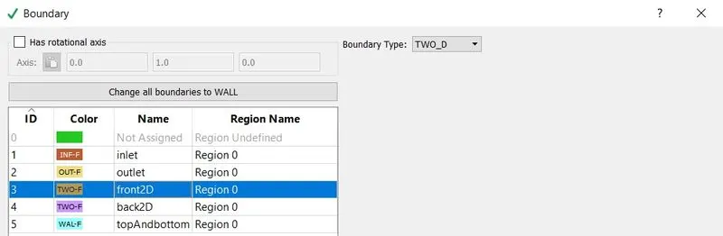
Front2D -
Boundary Type - TWO_D
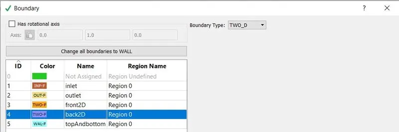
Back2D -
Boundary Type - TWO_D
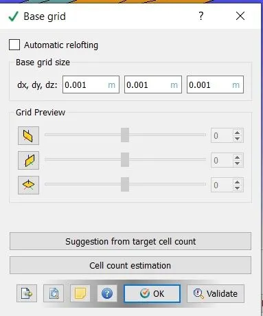
*In converge mesh generation is a fully automatic process.Converge uses cut cell method to generate the mesh.This is a patented method developed by coverge.
Base Grid = dx= 0.001 ; dy = 0.001 ; dz = 0.001 => ok
*As we want to moniter how flow behaves at the boundaries,we need to refine the mesh near the walls.To do that we will do
fixed embedding.
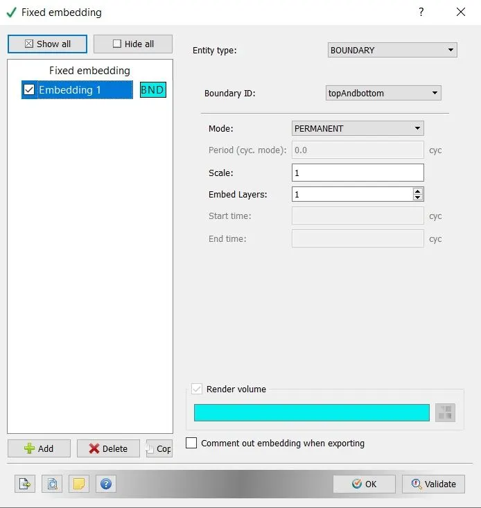
Boundary => Fixed Embedding => Add => Entitiy type boundary => Boundary ID topAndbottom => Mode Permanent => Scale 1 => Embed Layers 1.
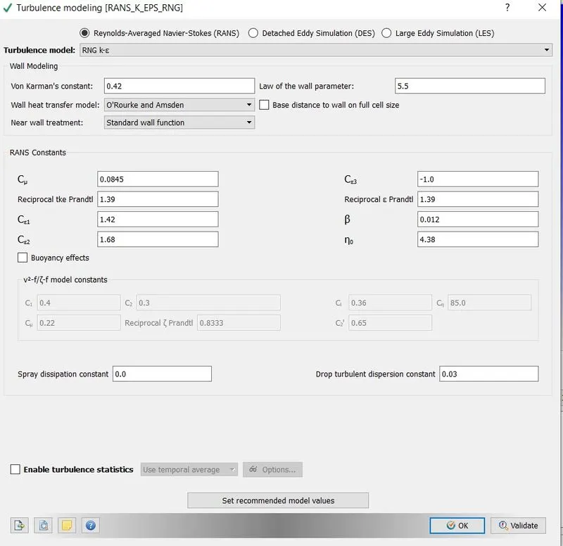
*For turbulence model select RNG `k-epsilon`
*In post variable selection,select the variables which needs to be post processed and set species mass fraction.
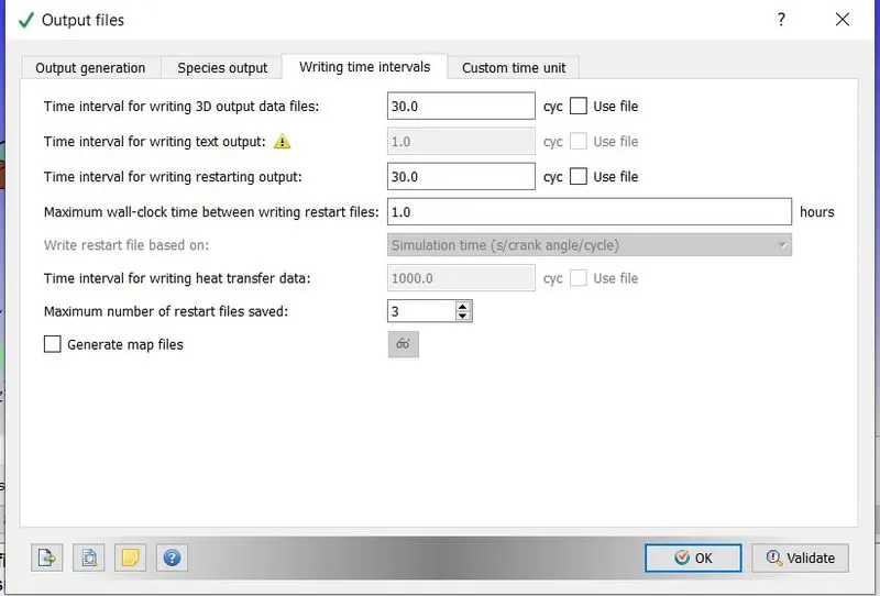
*We want our post processed graphes and animations to be smooth,so we want ample amount of ouput files.It is good practice to have at least 100 3D output files and same amount of text output files.
4.3] Solution :
*For running the simulation,first we need to export all the input files to the folder where we want to save our output files,
File => Export => Export Input Files => select the desired folder => Export.
*Now we will use CYGWIN command prompt to run our simulation.But before running the simulation first we need executables which willl solve the simulation,for that paste mpiexec.exe and converge.exe into the folder where we have exported all our input files.
*Now using CYGWIN command prompt,navigate to the folder where all the input files are exported,and type the below command,
mpiexec.exe -n 4 converge.exe restricted </dev/null> logfile &
*In the above command ,mpiexec.exe will help us to run our simulation in parallel,-n 4 are the number of cores on which we
want to run our simulation.As we are using the version of converge which has limit on the size of the file it can solve hence the command restricted.And the last part of the command dump all the data that is being generated into the logfile, which we can access during simulation procedure to see where our simulation has reached.
*The above command will create a folder named output containing all the generated 3D output data.As we will be using paraview as the postprocessing tool.Hence we need to convert these output files into the format that paraview can read.For this we will use converge post convert tool.
Go to converge post processing 3D =>give case name => select the file type => navigate to the output folder and select it
=> select all files => select all variables => convert.
This will create group file ,which will be used by paraview to post process our results.
4.4] Post Processing :
Case 1 => 2e-3 Mesh
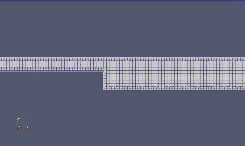
Fig = Mesh at 2e-3 Grid Spacing
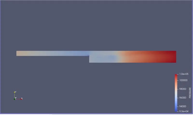
Fig = Pressure at 2e-3 Grid Spacing
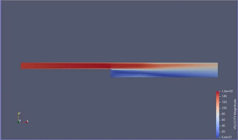
Fig = Velocity at 2e-3 Grid Spacing
Case 2 => 1.5e-3 Mesh
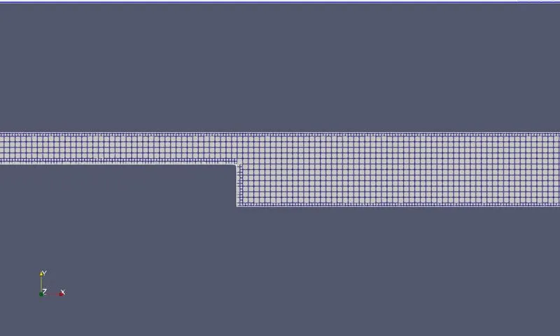
Fig = Mesh at 1.5e-3 Grid Spacing
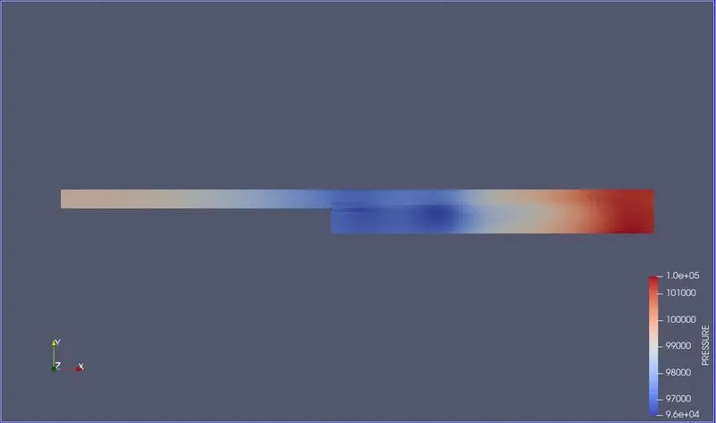
Fig = Pressure at 1.5e-3 Grid Spacing
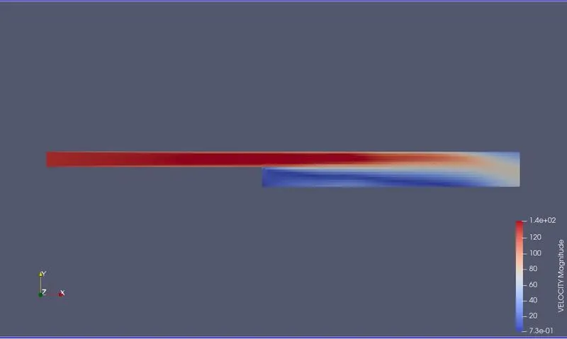
Fig = Velocity at 1.5e-3 Grid Spacing
Case 3 => 1e-3 Mesh
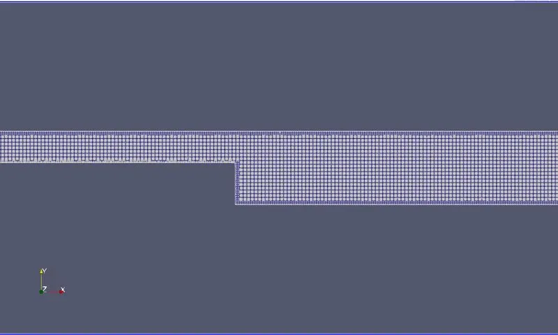
Fig = Mesh at 1e-3 Grid Spacing
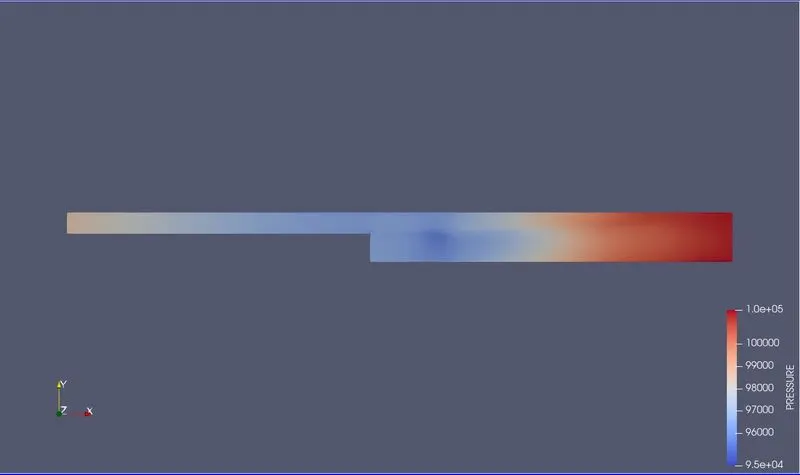
Fig = Pressure at 1e-3 Grid Spacing
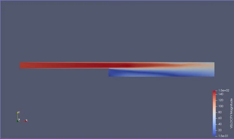
Fig = Velocity at 1e-3 Grid Spacing
5] Animations -
Case 1 - 2e-3Mesh
Velocity =>https://www.youtube.com/watch?v=i5umcYafMM8
Pressure =>https://www.youtube.com/watch?v=BsWxlNWTZ0g
Case2 -1.5e-3 Mesh
Velocity =>https://www.youtube.com/watch?v=m2wzX3N-_Vk
Pressure =>https://www.youtube.com/watch?v=jyUYocORAoY
Case 3 - 1e-3Mesh
Velocity =>https://www.youtube.com/watch?v=_wffud-xYMA
Pressure =>https://www.youtube.com/watch?v=0wvuLIU1dEM
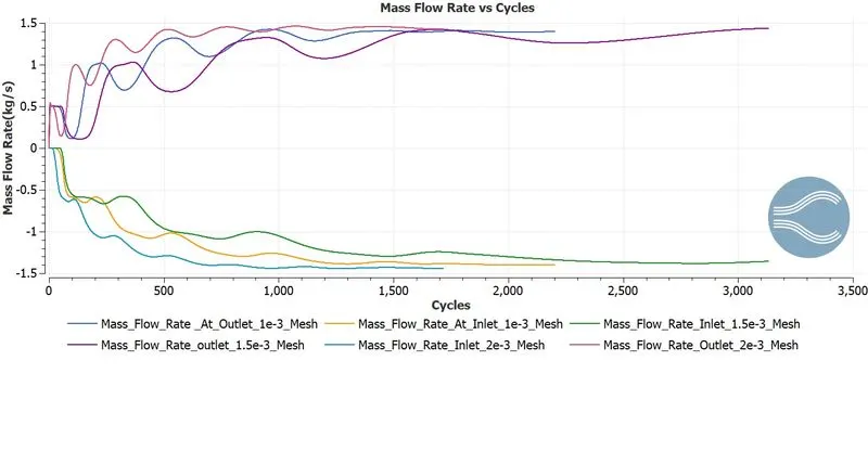
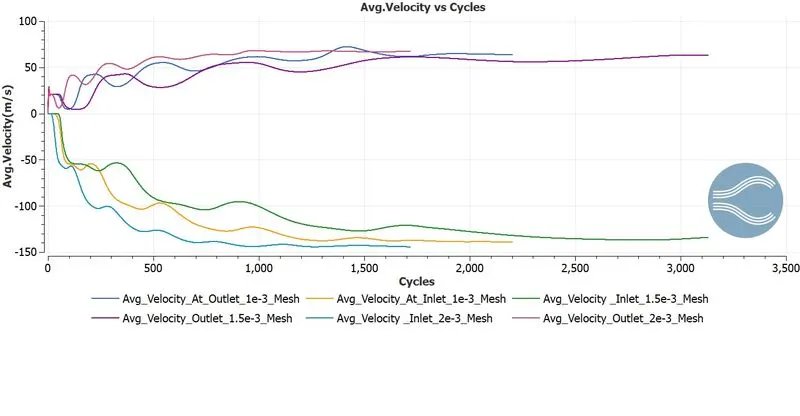
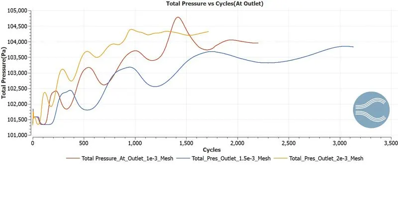
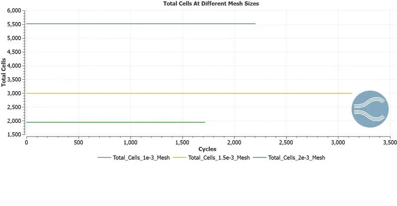
6] Variable Plots For Different Mesh Sizes -
7] Recirculation Region :
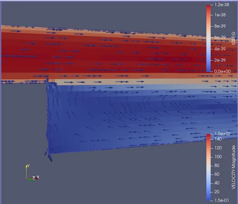
*Near the step in geometry,we can see the separation,this is due to boundary layer separation.Due to the change in an area,there is a pressure drop,which leads to the separation of the flow.The boundary layer separation is a phenomenon that occurs when fluid experiences a sudden change in area to the path of the flow.
*From the simulation performed itis clear that as the mesh becomes finner,number of cells increases and accuracy of the results increases.
*Pressure reduces at the inlet due to excessive momentum loss near the step wall.The flow separation resulting in a zonewith a pressure gradient called the recirculation zone.
| Grid Size | 2e-3 | 1.5e-3 | 1e-3 |
| Total Number of Cells | 1943 | 2994 | 5516 |
8] Conclusion :
*The mass flow rate at inlet and outlet is conserved.
*The average velocity at inlet is higher than outlet,as there is pressure drop at the step region,thus vortex generates and velocity at outlet decreases.
*RNG `k-epsilon` turbulence model is used to capture the boundary layer effectively.