Week 1- Mixing Tee

Mixing Tee

Aim: To set up steady-state simulations to compare the mixing effectiveness when hot inlet temperature is 36⁰C & the Cold inlet is at 19⁰C. by using two version of the mixing tee.

Objective:

• To set up steady-state simulations to compare the mixing effectiveness when hot inlet temperature is 36⁰C & the Cold inlet is at 19⁰C.
• Use the k-epsilon and k-omega SST model for the first case and based on your judgement use the more suitable model for further cases. Giving the reason for choosing a suitable model is compulsory.

1. Case 1
   • Short mixing tee with a hot inlet velocity of 3m/s.
   • Momentum ratio of 2, 4.
2. Case 2
   • Long mixing tee with a hot inlet velocity of 3m/s.
   • Momentum ratio of 2, 4.

• Momentum ratio = velocity at cold inlet / velocity at hot inlet
• In a table, compare the following values from the 2 cases.

1. Cell count
2. Average outlet temperature
3. Number of iterations for convergence

Procedure:

Introduction: In this type of project is used in air conditioning application where the desired temperature is required to maintain due to that purpose we do the study and choose best optimum model for such application.

Step 1 ) Pre- processing :-

• Geometry : First we take the solid geometry in the ansys spaceclaim and convert it into desirable cad model.

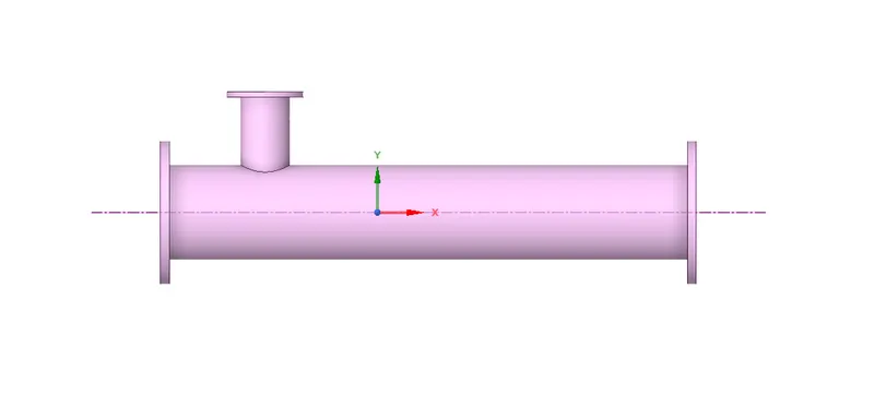
• The above figure shows the 3d solid geometry of short tee.

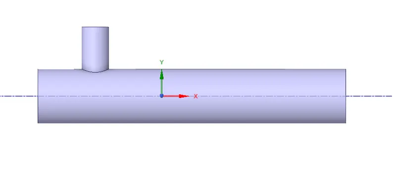
• The above figure shows the 3d cad model of short tee which are taking for simulation.

Step 2) Mesh :The next step is to take this model for meshing

• Before meshing we give the name for boundaries by using cltr+F for selecting the face and give the appropriate name for the face

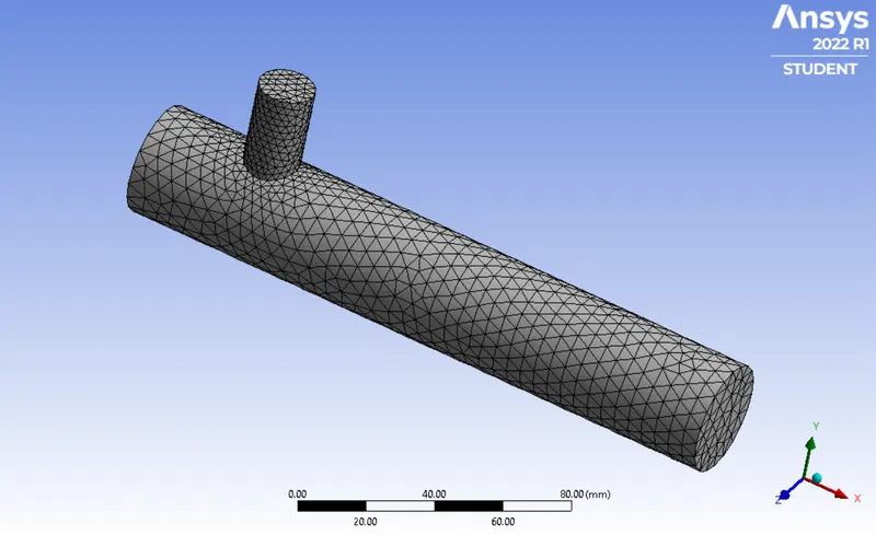
• Given boundary names which is shown in named selections and mesh shown right side of image
• To get the converged results we need good quality of mesh with good quality of mesh elements
• Here below image we can see that the quality of the mesh element in mesh metric

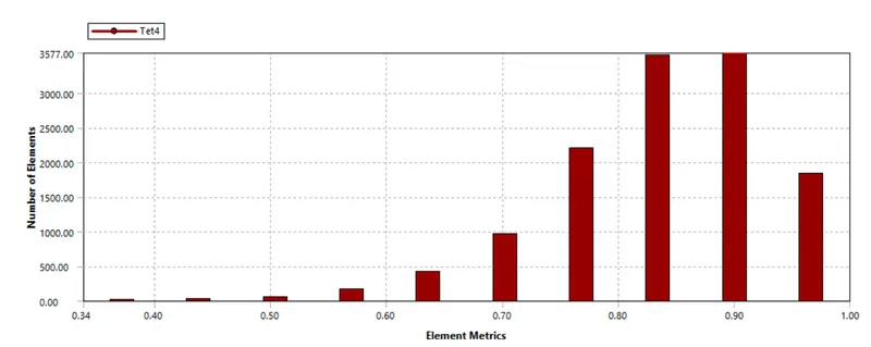
Elemental quality of mesh

• Here we can see that the more number of elements quality is good and all elements quality is above 34% ,so we can use this mesh for further study .

Step 3) Set up and solution:

• Here we use the ansys fluent,open the set up window then the fluent is open.
• First we can check mesh and evaluate the quality of mesh ,for changing the units of variable we can go to the units and change it ,here we use unit for temperature is celsius.
• In setting up physics, I select steady state because here we are solving the steady state equation and we use pressure based type,Velocity formulation is absolute.
• On the energy equation we can choose the turbulence model here .
• We use the material for flow is air so we check this is in material section.
• Next we check the cell zone condition in that check the material is air .
• The important step is to give boundary conditions and according to momentum ratio we give the values of velocity of air for inlets and given temperature of air for inlet.
• Next step is to define solution parameter,here we use hybrid method.
• In order to get the report of the simulation and give the monitor for the required variable we use definition section
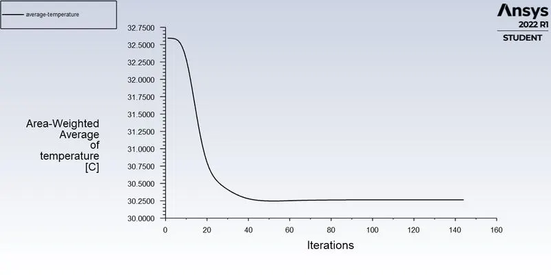
• Here we want the outlet temperature so we use the surface report in that area weighted average report,Due to that average temperature is computed,and also use standard deviation report for knowing the actual deviation of temperature .

Step 4) Result : Post processing :

• After solution,the last step is post processing to know the result.
• Here the major focus on temperature and velocity contour plot along and across the pipe.
• Line plot for both temperature and velocity along and across the length of the pipe.
• We can check the result for all the cases below.

Selection of Turbulance model :

• Case 1
  • Short mixing tee with a hot inlet velocity of 3m/s.
  • Momentum ratio of 2, 4.
• 1st we take short mixing tee and momentum ratio 2 and use k-epsilon and k-omega SST model and after analysis we use best suitable model for the next case simulation.
• In this simulation we use velocity of hot inlet is 3 m/sec and cold inlet is 6m/sec and given temperature of hot inlet is `36^0`,and cold inlet is `19^0`
• 1st we use k-epsilon model.

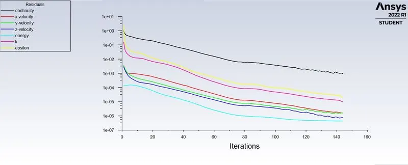
Fig(1) Residual plot for momentum ratio 2 using k-epsilon model :

fig(2) Area weighted average of temperature plot for momentum ratio 2 using k-epsilon model:

fig(3) Standard deviation of temperature plot for momentum ratio 2 using k-epsilon model:

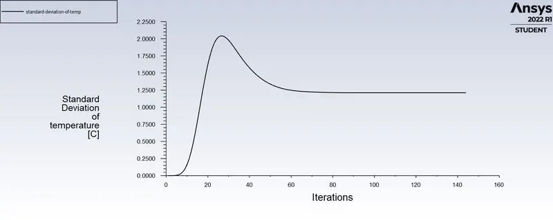
Fig (4) Temperature contour plot on cut plane (plane XY) along the pipe for momentum ratio 2 using k-epsilon model:

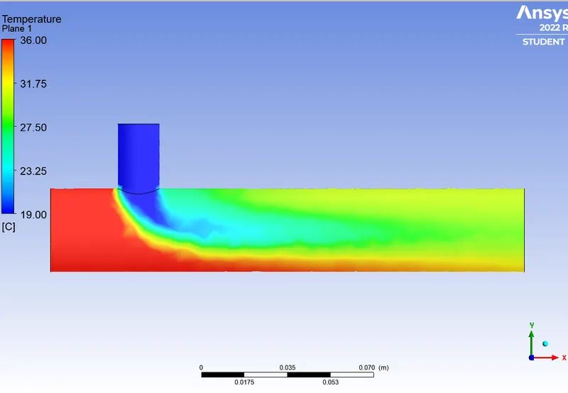
Fig (5) Velocity contour plot on cut plane (plane XY) along the pipe for momentum ratio 2 using k-epsilon model:

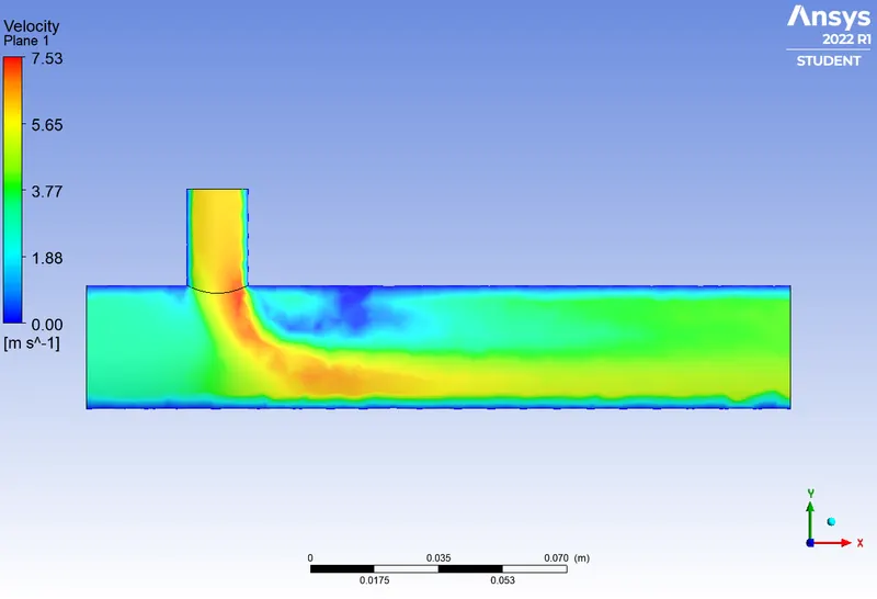
Fig (6) Temperature contour plot on cut plane across the pipe for momentum ratio 2 using k-epsilon model:

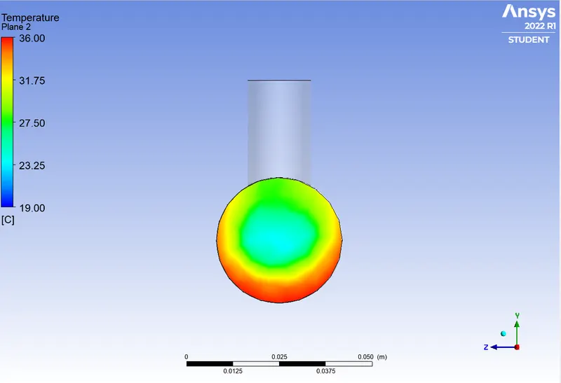
Fig (6) Velocity contour plot on cut plane across the pipe for momentum ratio 2 using k-epsilon model:

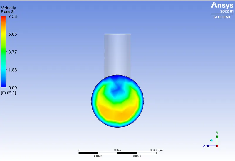
Fig (7) Temperature line plot along the length of pipe for momentum ratio 2 using k-epsilon model:

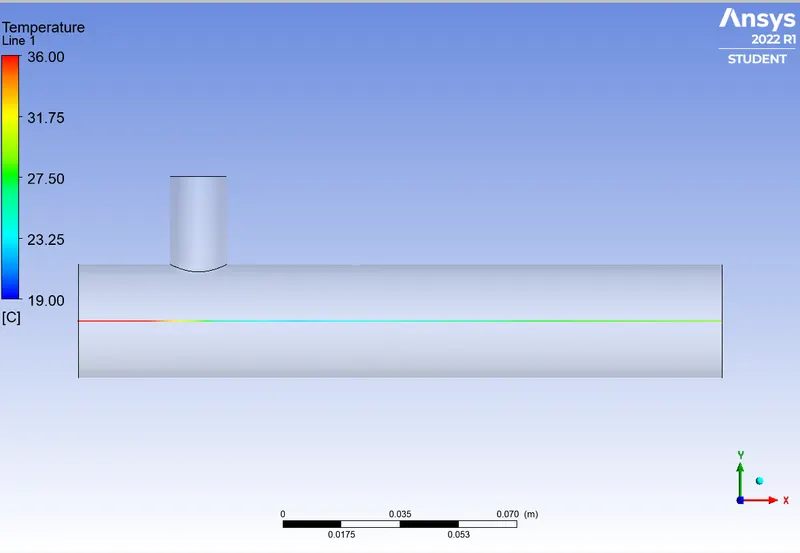
Fig (8) Velocity line plot along the length of pipe for momentum ratio 2 using k-epsilon model:

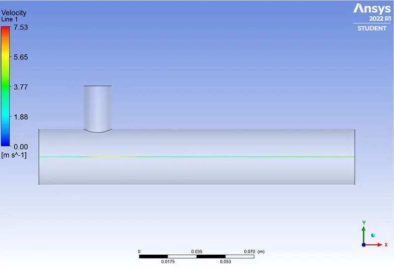
Fig (9) Temperature line plot across the length of pipe for momentum ratio 2 using k-epsilon model:

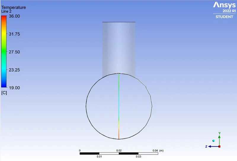
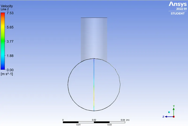
Fig (10) Velocity line plot across the length of pipe for momentum ratio 2 using k-epsilon model:

• Here we use K-omega model for short tee momentum ratio 2 and their result plots are below:

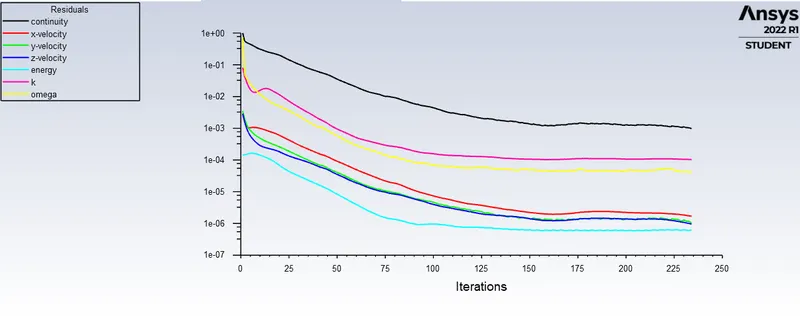
Fig(11) Residual plot for momentum ratio 2 using k-omega model :

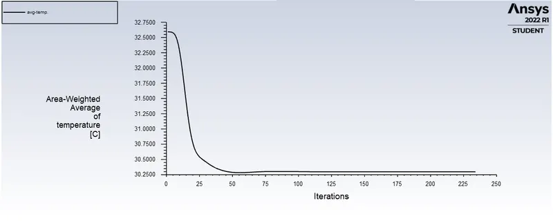
fig(12) Area weighted average of temperature plot for momentum ratio 2 using k-omega model:

fig(13) Standard deviation of temperature plot for momentum ratio 2 using k-omega model:

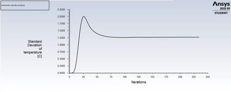
Fig (14) Temperature contour plot on cut plane (plane XY) along the pipe for momentum ratio 2 using k-omega model:

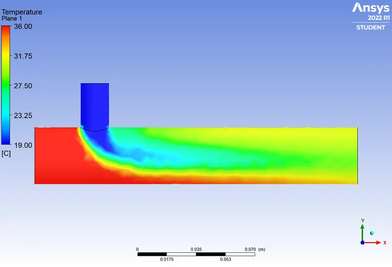
Fig (15) Velocity contour plot on cut plane (plane XY) along the pipe for momentum ratio 2 using k-omega model:

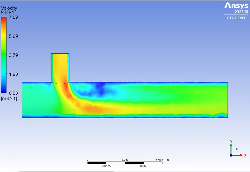
Fig (16) Temperature contour plot on cut plane across the pipe for momentum ratio 2 using k-omega model:

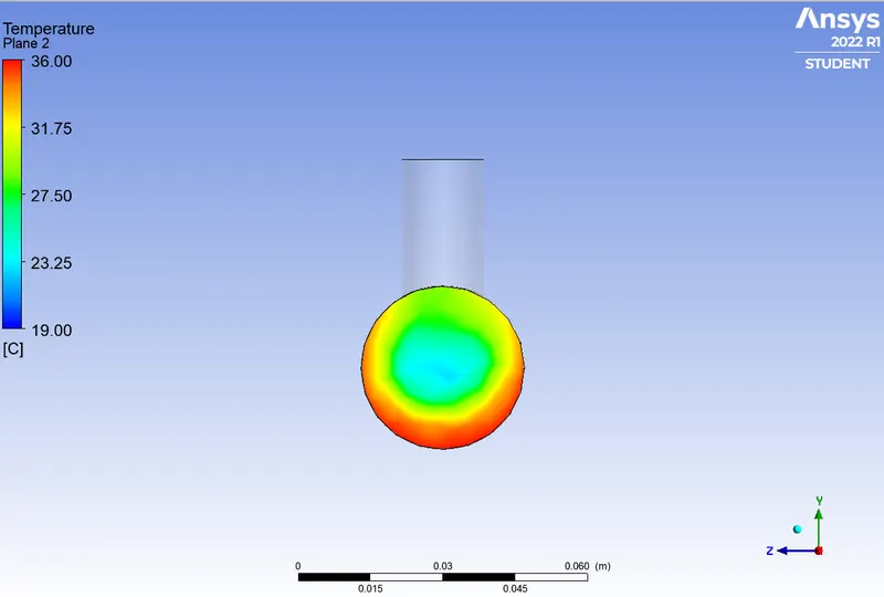
Fig (17) Velocity contour plot on cut plane across the pipe for momentum ratio 2 using k-omega model:

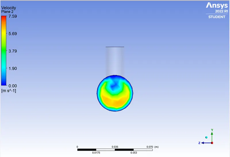
Fig (18) Temperature line plot along the length of pipe for momentum ratio 2 using k-omega model:

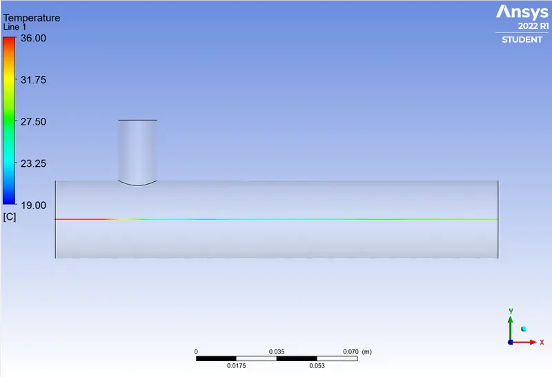
Fig (19) Velocity line plot along the length of pipe for momentum ratio 2 using k-omega model:

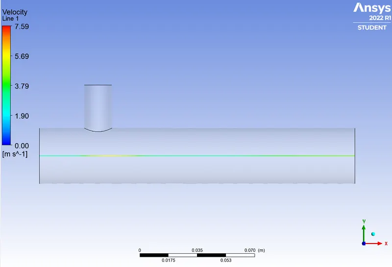
Fig (20) Temperature line plot across the length of pipe for momentum ratio 2 using k-omega model:

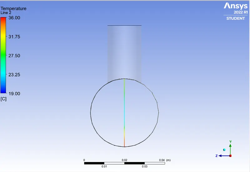
Fig (21) Velocity line plot across the length of pipe for momentum ratio 2 using k-omega model:

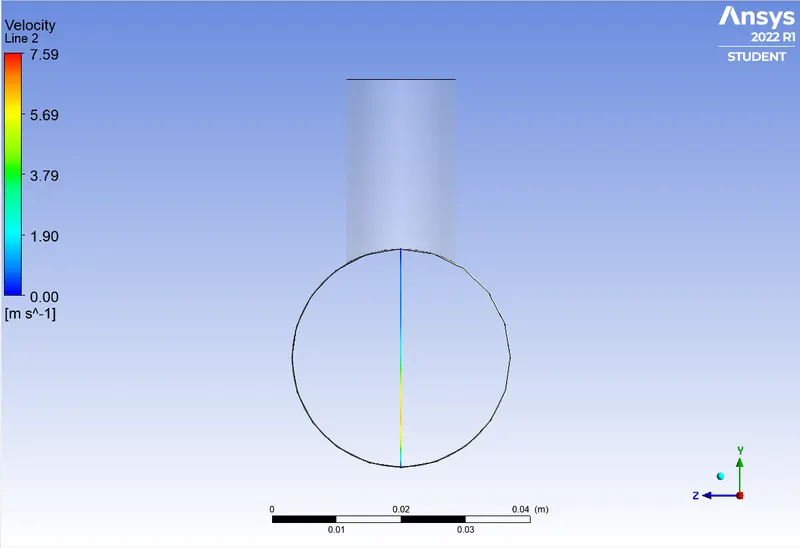
• We take short mixing tee and momentum ratio 4 and use k-epsilon and k-omega SST model and after analysis we use best suitable model for the next case simulation.
• In this simulation we use velocity of hot inlet is 3 m/sec and cold inlet is 12m/sec and given temperature of hot inlet is `36^0`,and cold inlet is `19^0`
• 1st we use k-epsilon model.

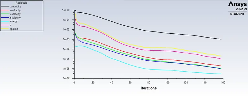
Fig(22) Residual plot for momentum ratio 4 using k-epsilon model :

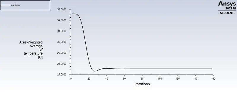
fig(23) Area weighted average of temperature plot for momentum ratio 4 using k-epsilon model:

fig(24) Standard deviation of temperature plot for momentum ratio 4 using k-epsilon model:

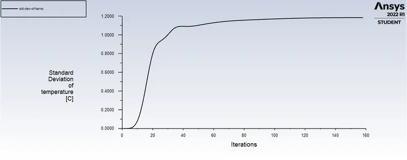
Fig (25) Temperature contour plot on cut plane (plane XY) along the pipe for momentum ratio 4 using k-epsilon model:

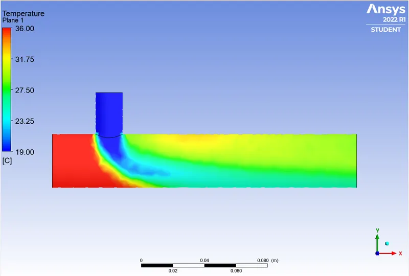
Fig (26) Velocity contour plot on cut plane (plane XY) along the pipe for momentum ratio 4 using k-epsilon model:

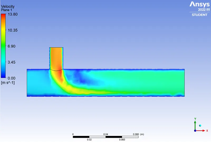
• Here we use K-omega model for short tee momentum ratio 4 and their result plots are below:

Fig(27) Residual plot for momentum ratio 4 using k-omega model :

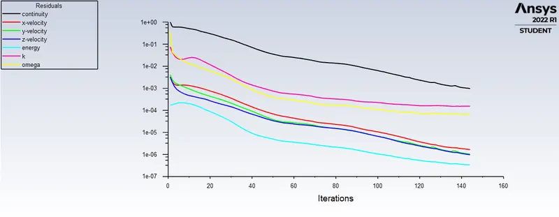
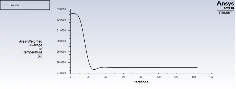
fig(28) Area weighted average of temperature plot for momentum ratio 4 using k-omega model:

fig(29) Standard deviation of temperature plot for momentum ratio 4 using k-omega model:

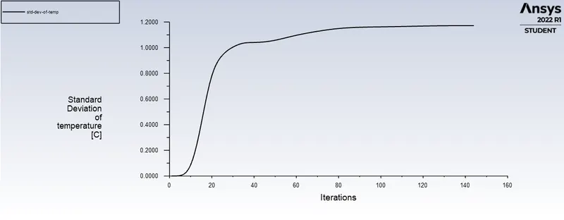
Fig (30) Temperature contour plot on cut plane (plane XY) along the pipe for momentum ratio 4 using k-omega model:

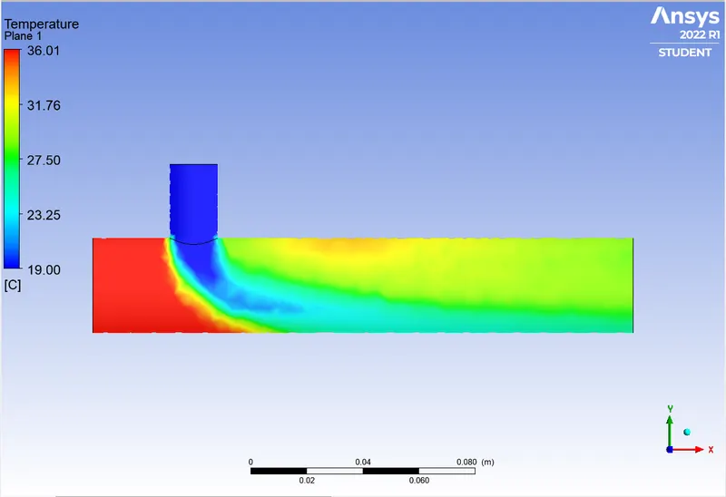
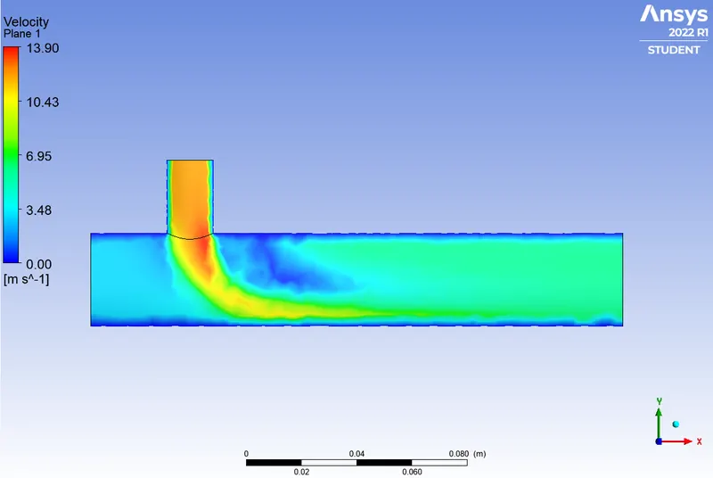
Fig (31) Velocity contour plot on cut plane (plane XY) along the pipe for momentum ratio 4 using k-omega model:

We have used both the turbulance model for simulation of case 1,For comparison all the results are tabulated as follows:

Sr No	Model used	Cell count	Momentum ratio	Turbulance model	Average temperature at outlet	Standard Deviation of temp.	Number of iteration
1	Short Tee	12787	2	k-epsilon	30.2640	1.2106	142
2	Short Tee	12787	2	k-omega	30.2980	1.2696	234
3	Short Tee	12787	4	k-epsilon	27.5409	1.1834	158
4	Short Tee	12787	4	k-omega	27.5306	1.1721	144

From the above result we observed that in momentum ratio 2 the k-epsilon model take less time for converging the result and the number of iteration required for converging is also less than the k-omega model So we decided to use k-epsilon model for simulation of case2.

Case 2

• Long mixing tee with a hot inlet velocity of 3m/s.
• Momentum ratio of 2, 4.
• In this simulation 1st we simulate for momentum ratio 2

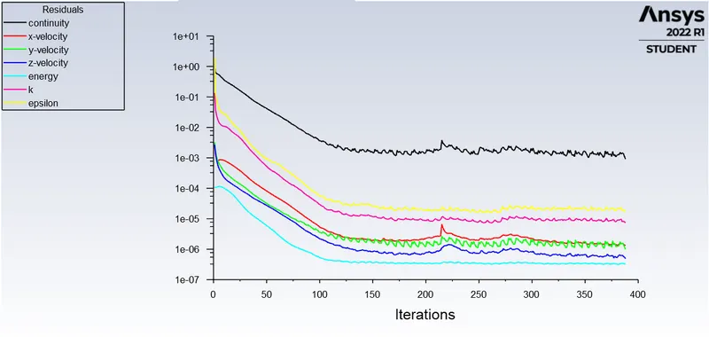
Fig(32) Residual plot for momentum ratio 2 using k-epsilon model :

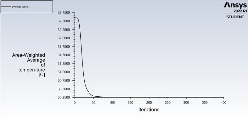
fig(33) Area weighted average of temperature plot for momentum ratio 2 using k-epsilon model:

fig(34) Standard deviation of temperature plot for momentum ratio 2 using k-epsilon model:

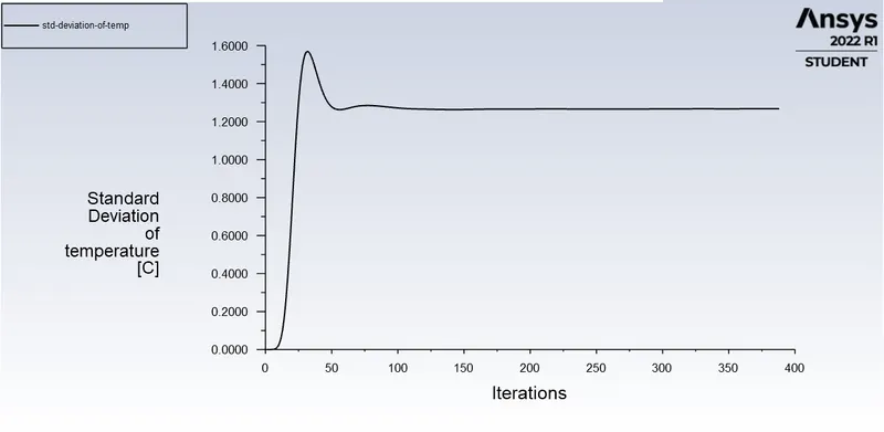
Fig (35) Temperature contour plot on cut plane (plane XY) along the pipe for momentum ratio 2 using k-epsilon model:

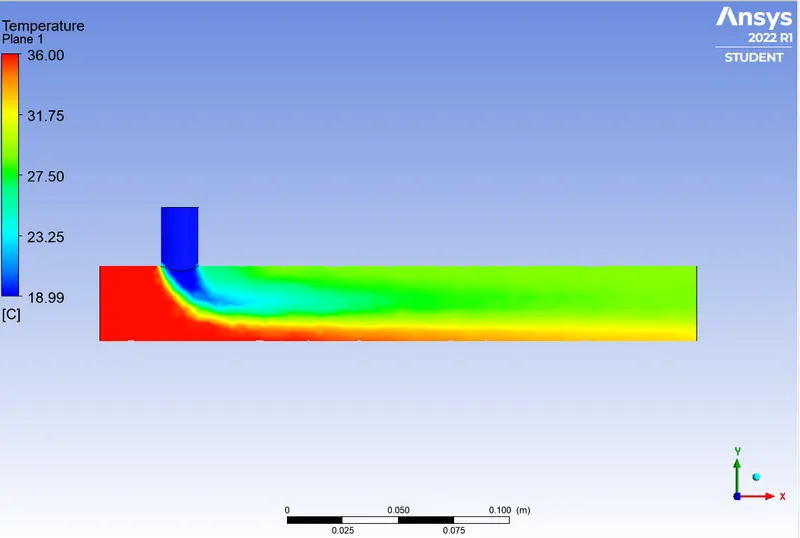
Fig (36) Velocity contour plot on cut plane (plane XY) along the pipe for momentum ratio 2 using k-epsilon model:

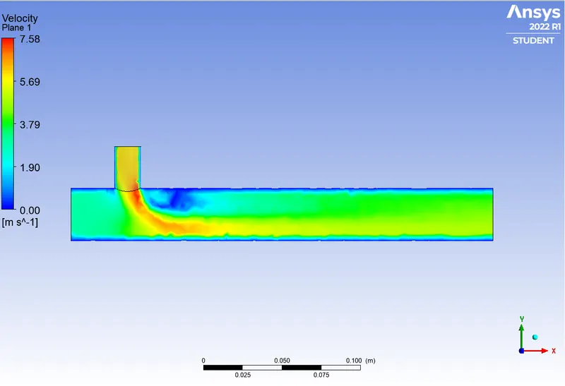
Fig (37) Temperature contour plot on cut plane across the pipe for momentum ratio 2 using k-epsilon model:

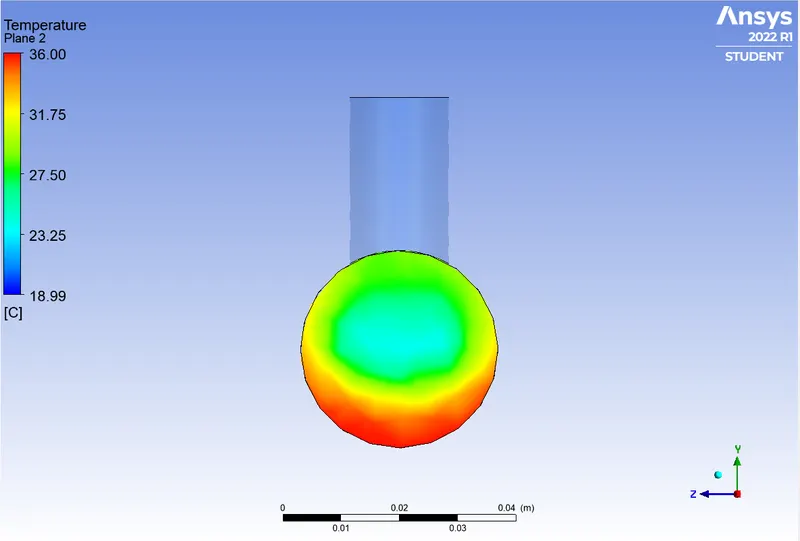
Fig (38) Velocity contour plot on cut plane across the pipe for momentum ratio 2 using k-epsilon model:

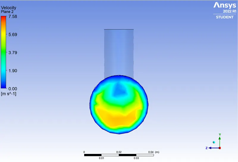
Fig (39) Temperature line plot along the length of pipe for momentum ratio 2 using k-epsilon model:

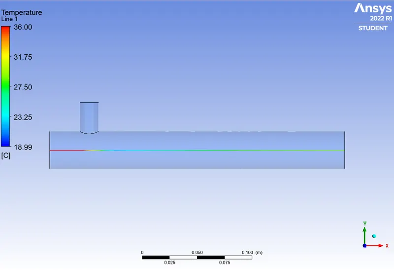
Fig (40) Velocity line plot along the length of pipe for momentum ratio 2 using k-epsilon model:

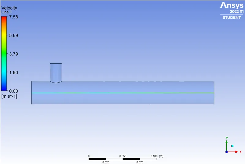
Fig (41) Temperature line plot across the length of pipe for momentum ratio 2 using k-epsilon model:

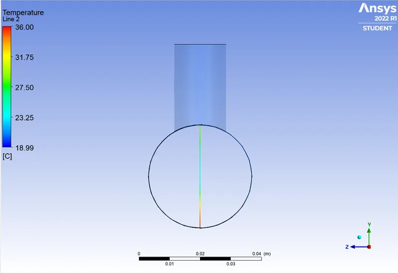
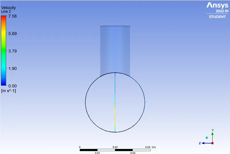
Fig (42) Velocity line plot across the length of pipe for momentum ratio 2 using k-epsilon model:

We simulte the long mixing tee for momentum ratio 4 using k-epsilon model and their results are shown below:

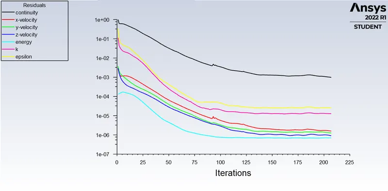
Fig(43) Residual plot for momentum ratio 4 using k-epsilon model :

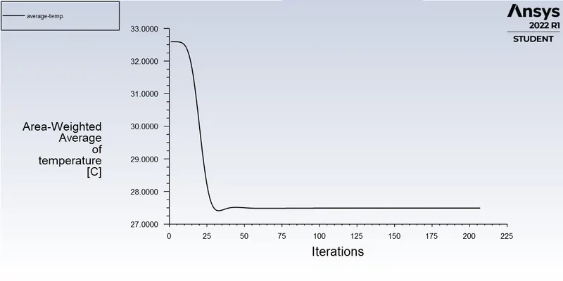
fig(44) Area weighted average of temperature plot for momentum ratio 4 using k-epsilon model:

fig(45) Standard deviation of temperature plot for momentum ratio 4 using k-epsilon model:

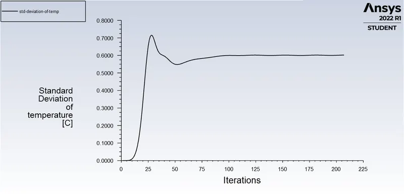
Fig (46) Temperature contour plot on cut plane (plane XY) along the pipe for momentum ratio 4 using k-epsilon model:

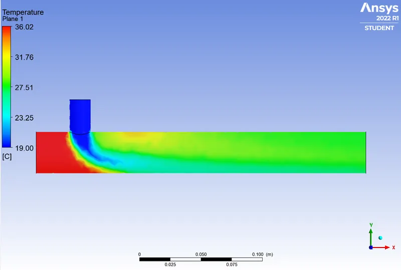
Fig (47) Velocity contour plot on cut plane (plane XY) along the pipe for momentum ratio 4 using k-epsilon model:

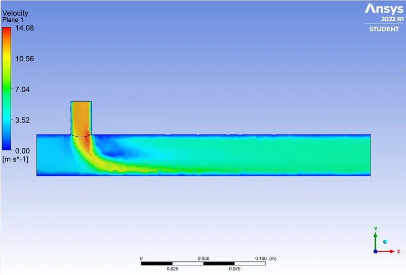
Fig (48) Temperature contour plot on cut plane across the pipe for momentum ratio 4 using k-epsilon model:

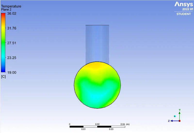
Fig (49) Velocity contour plot on cut plane across the pipe for momentum ratio 4 using k-epsilon model:

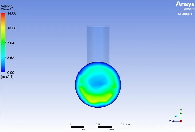
Fig (50) Temperature line plot along the length of pipe for momentum ratio 4 using k-epsilon model:

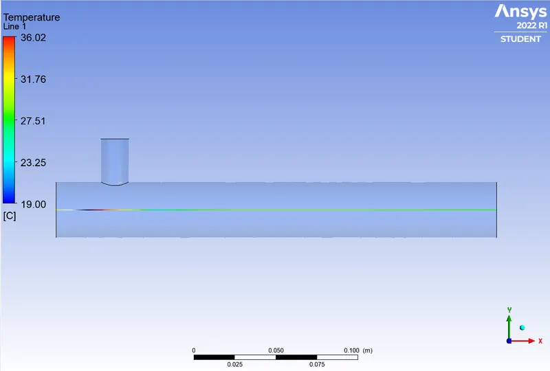
Fig (51) Velocity line plot along the length of pipe for momentum ratio 4 using k-epsilon model:

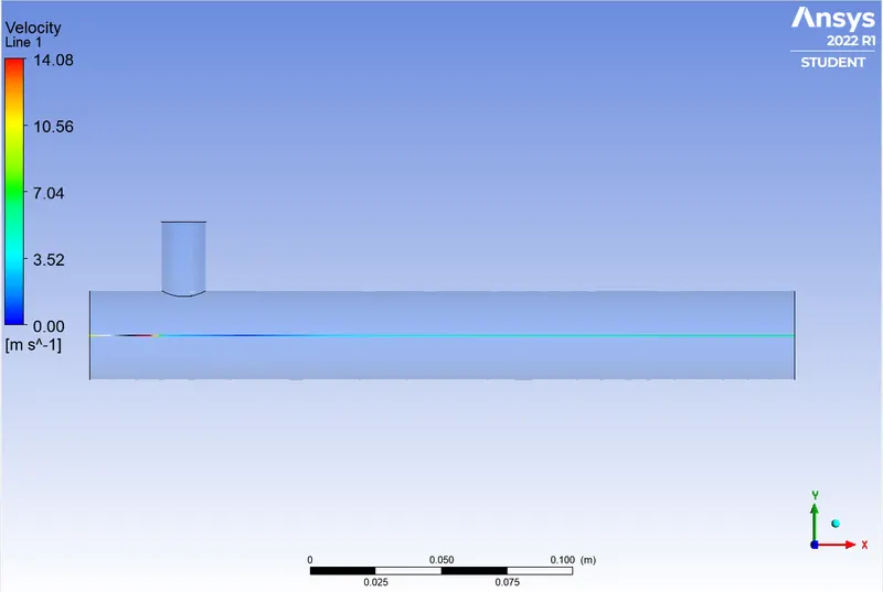
Fig (52) Temperature line plot across the length of pipe for momentum ratio 4 using k-epsilon model:

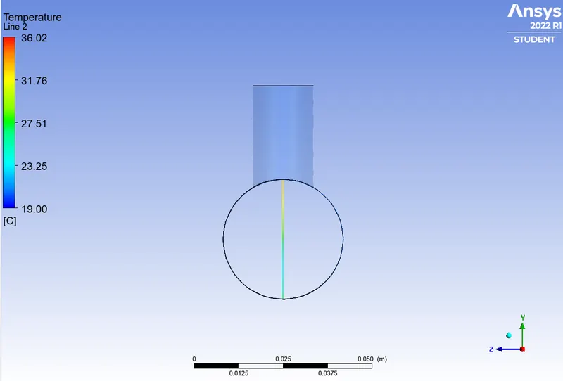
Fig (53) Velocity line plot across the length of pipe for momentum ratio 4 using k-epsilon model:

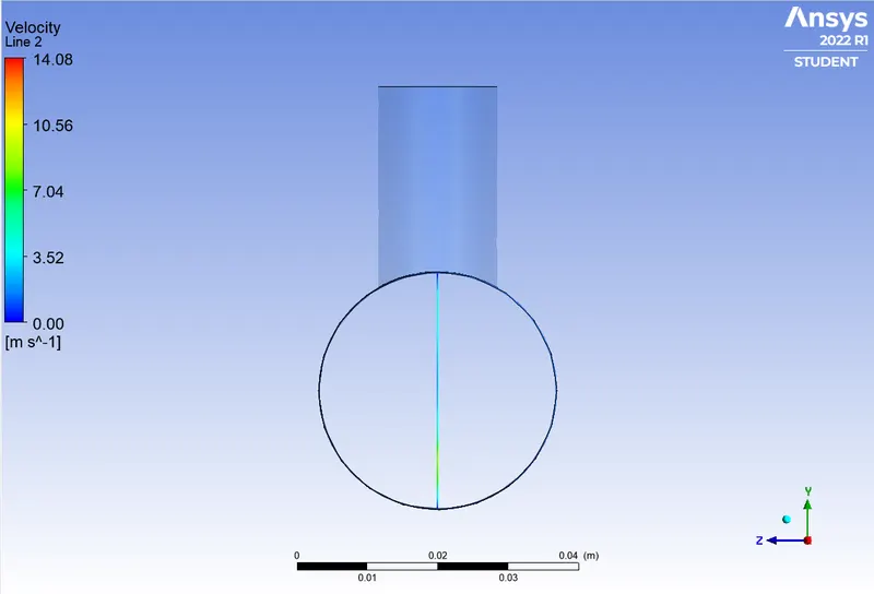
• Case 2) Results are tabulated as follows:

Sr No	Model used	Cell count	Momentum ratio	Turbulance model	Average temperature at outlet	Standard Deviation of temp.	Number of iteration
1	Long tee	15648	2	k-epsilon	30.2592	1.2672	388
2	Long Tee	15648	4	k-epsilon	27.4922	0.6020	207

Mesh Independent Study :

For mesh independence test we select case 1) short tee momentum ratio 2 and we do the study for mesh element size 7mm,5mm,3mm :

1) Mesh element size: 7mm

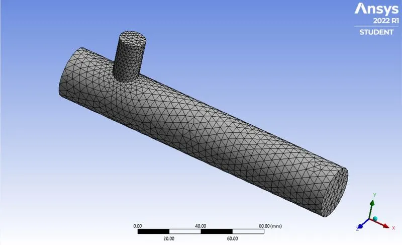
Above fig shows the generated mesh of size 7mm

• Residual plot:

• Area weighted average Temperature plot:

• Standard Deviation of temperature plot:

2) Mesh element size: 5 mm

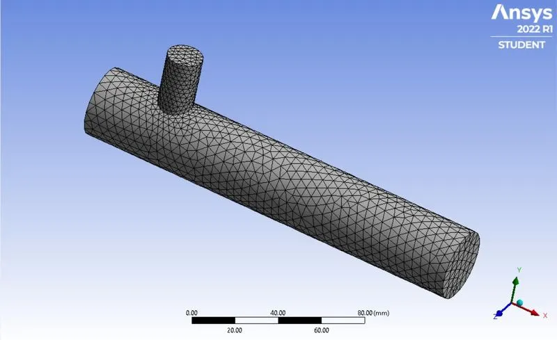
Above fig shows the generated mesh of size 5 mm

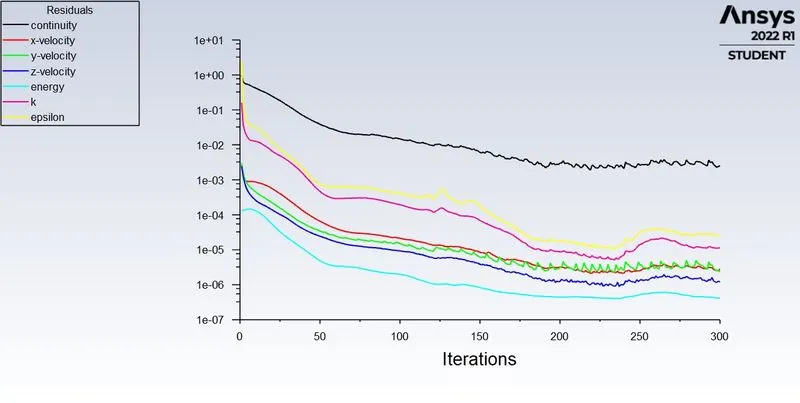
• Residual plot:

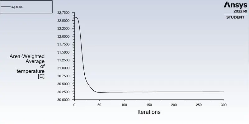
• Area weighted average Temperature plot:

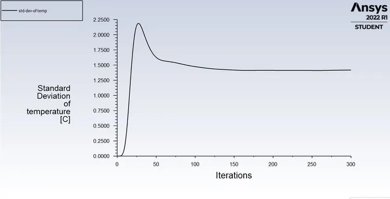
• Standard Deviation of temperature plot:

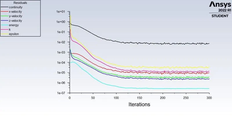
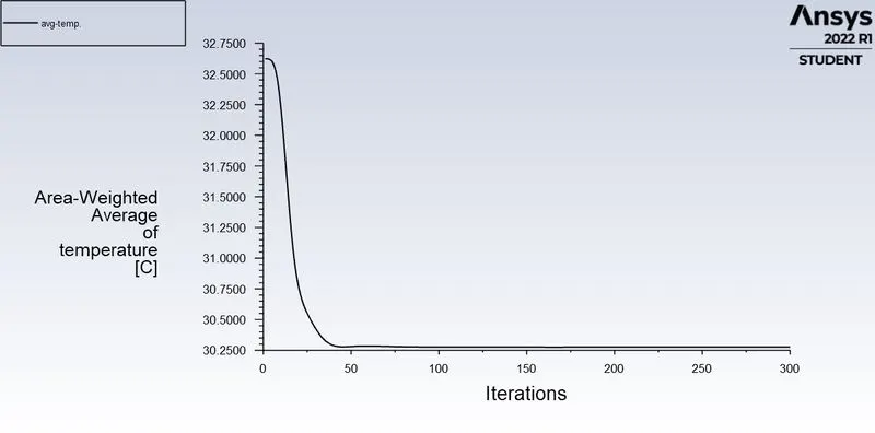
3) Mesh element size: 3 mm

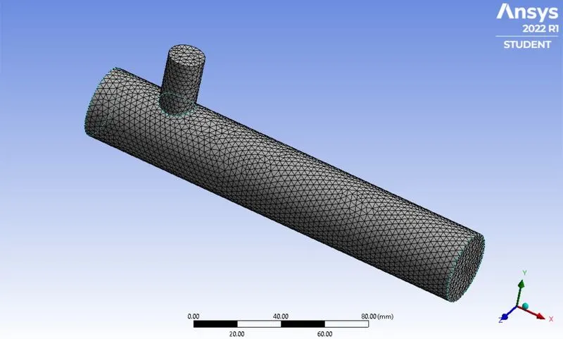
Above fig shows the generated mesh of size 3 mm

• Residual plot:

• Area weighted average Temperature plot:
• Standard Deviation of temperature plot:

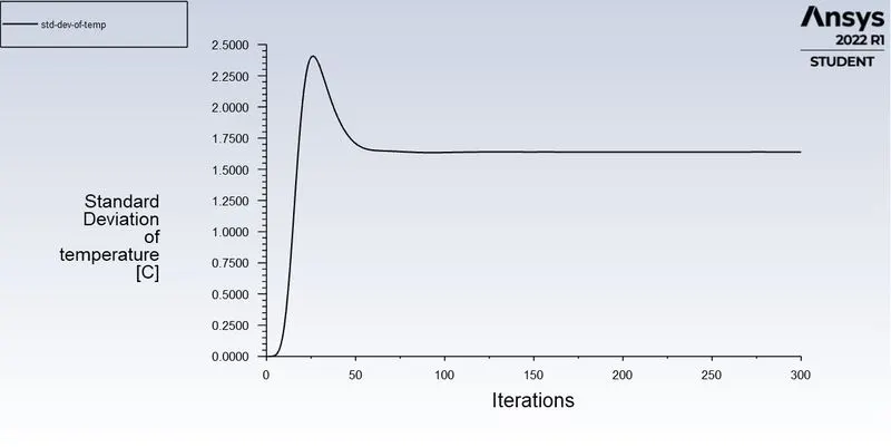
Results of Mesh independent study are tabulated as follows:

Sr No	Mesh element size	Cell count	Average temperature at outlet	Standard Deviation of temp.	Number of iteration
1	7mm	12787	30.264	1.21	142
2	5mm	14249	30.247	1.41	300
3	3mm	39792	30.2763	1.63	300

• From the above mesh independent study result we observed that their is no large variation in output results so we decided to use 7 mm size for the simulation of mixing tee case 1 and case 2 .

Conclusion:

Effect of length and momentum ratio on results:

• From the results of both the cases we can say that the output temperature is independent on length of mixing tee.
• Momentum ratio affects on outlet temperature ,If momentum ratio increases then the outlet temperature is dropping suddenly.