Week 4 - CHT Analysis on Exhaust port

Aim : To perform the steady state conjugate heat transfer simulation on exhaust port.

Objective :

• Describe in brief why and where a CHT analysis is used?
• Maintain the y+ value according to the turbulence model and justify the results.
• Calculate the wall/surface heat transfer coefficient on the internal solid surface & show the velocity & temperature contours in appropriate areas.
• How would you verify if the HTC predictions from the simulations are right? On what factors does the accuracy of the prediction depend on?

Procedure:

• CHT Analysis:
• Conjugate heat transfer (CHT) analysis can accurately predict heat transfer by simultaneous solving all the relevant solid and flow field heat transfer processes, for example: conduction through solids, free and forced convection in the gases/fluids and thermal radiation.
• The CHT approach has an advantage over FEA thermal analysis.in that wall heat transfer coefficients and their local variations on surfaces are directly calculated within the model rather than based on simplified empirical calculations.
• The CHT approach therefore has benefits for those applications where heat transfer is either non-uniform or difficult to calculate empirically.

Applications of CHT analysis:

• Typical applications of this analysis type exist as, but are not limited to, the simulation of heat exchangers, cooling of electronic equipment, and general-purpose cooling and heating systems.

Simulation on baseline mesh :

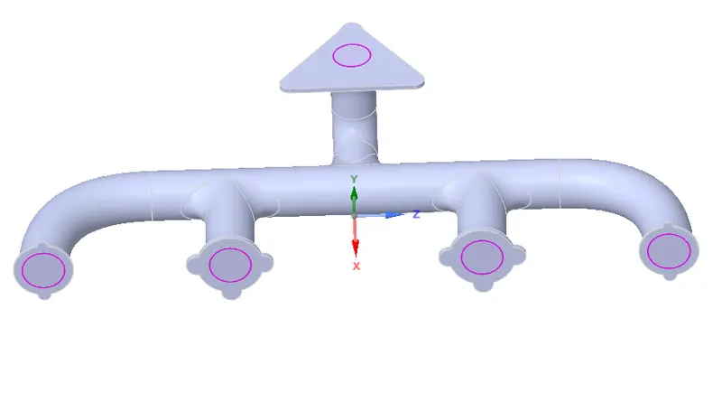
• Geometry : The geometry used for Analysis is shown in fig below:

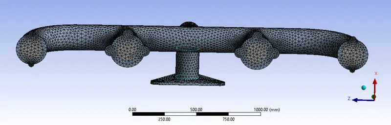
Mesh:

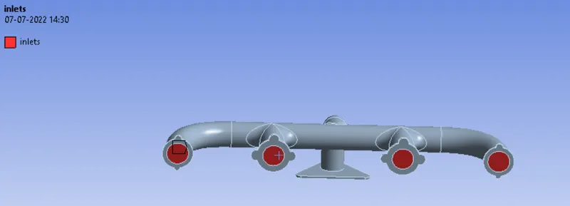
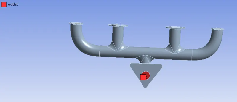
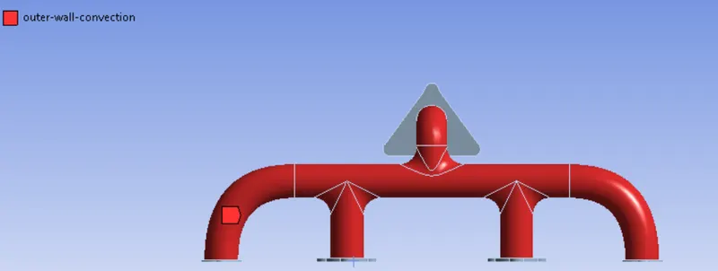
Give the names to the boundaries :

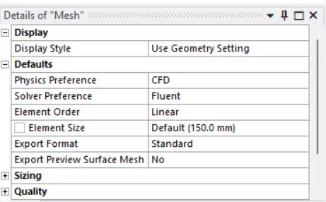
Mesh Size :

Mesh :

Set Up :

Solver Type: Pressure based

Velocity formulation: Absolute

Time: Steady state

Viscous Model: K epsilon

Material : for fluid : Air ,

For solid surface: Aluminium

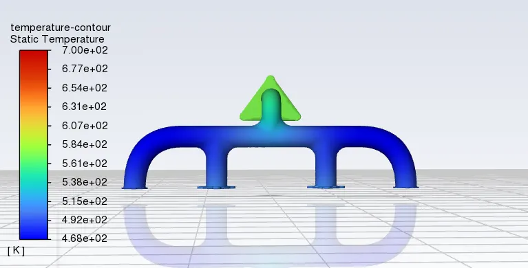
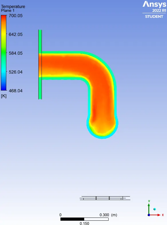
Boundaries : inlet : Velocity : 5 m/sec , Temperature : 700K

outlet: Gauge pressue [pa]: 0

outer wall convection: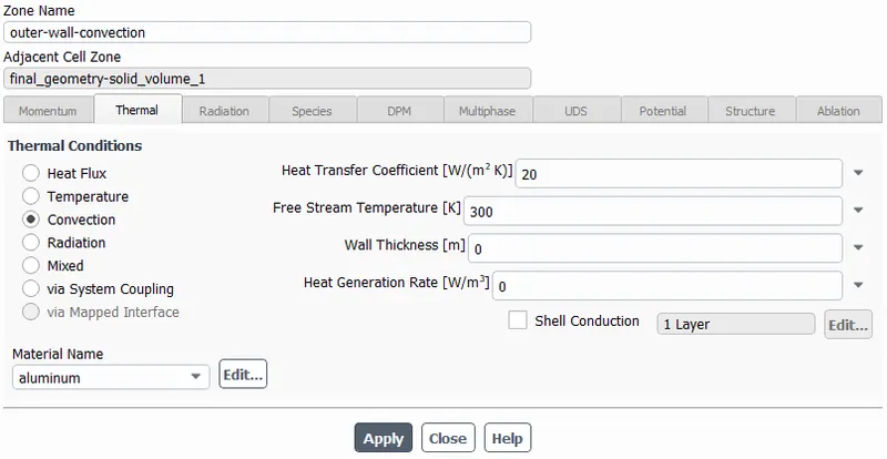

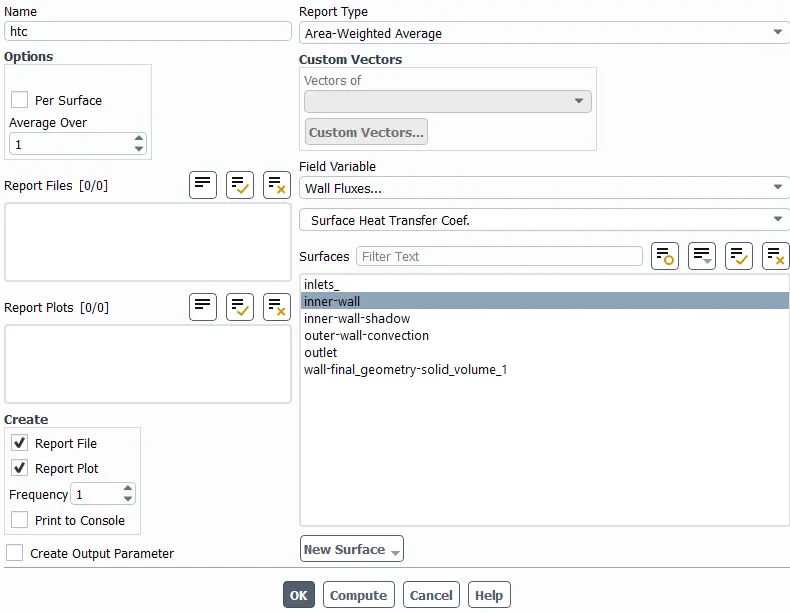
Solution: We want heat transfer coefficient at inner wall due to that we create report

Results :

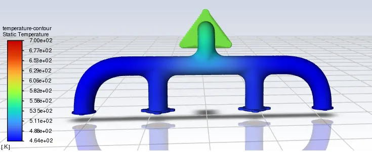
Create contour `rarr`Temperature`rarr` Field Variable `rarr`All Named Selections

Create contour `rarr` Velocity `rarr`Field Variable `rarr` All Named Selections

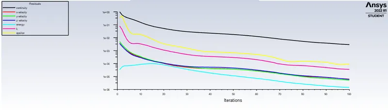
For 100 iterations we calculate the results:

Result:

Residual plot:

Temperature contour plot:

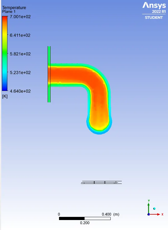
Temperature plot in XY plane :

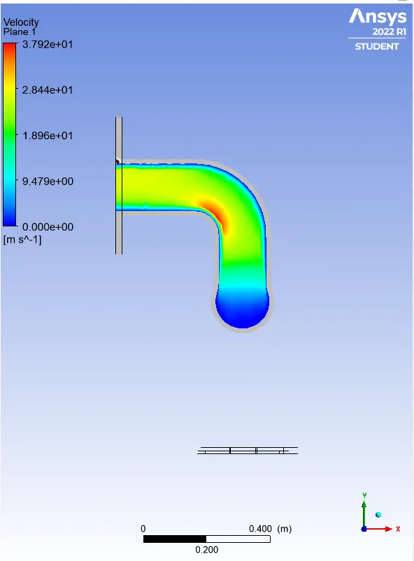
Velocity plot in XY plane :

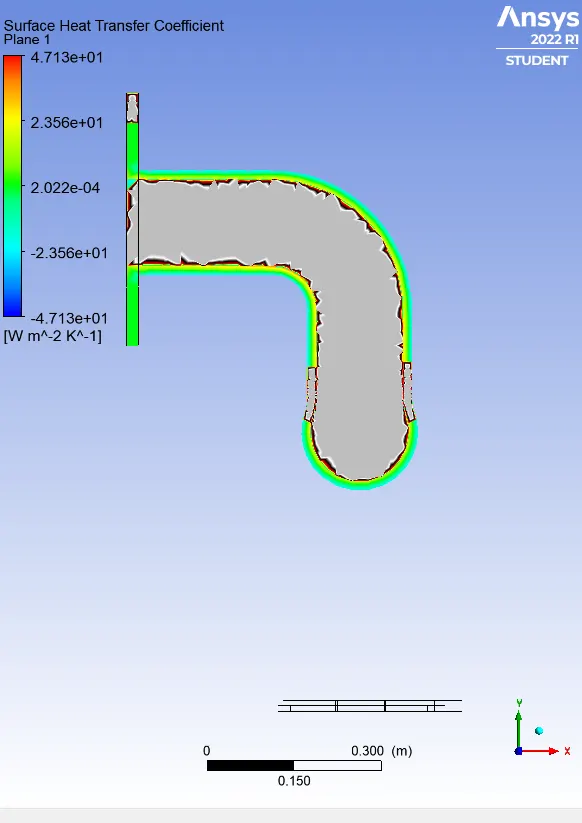
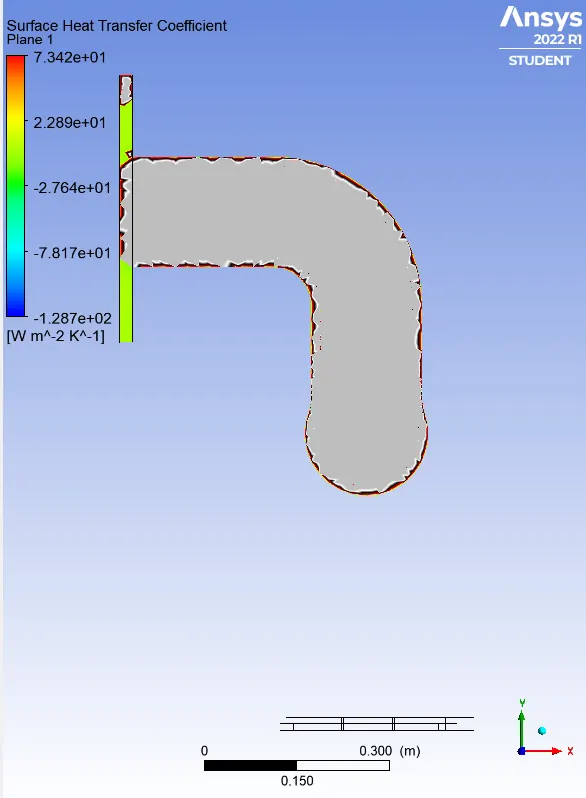
Surface Heat Transfer Coefficient in XY plane :

Simulation on Refined mesh:

The outer wall is refined by using element size 40mm , and we use 8 inflation layer to capture the flow accurately.

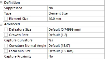
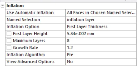
We calculate first layer thickness height for y+ value is 1 because we want to capture the flow near the wall for that we use k omega turbulance model for simulation.

Generated Mesh:

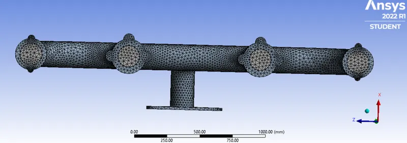
Setup and solution: All the process is same but the turbulance model is changed to K-omega SST in this simulation.

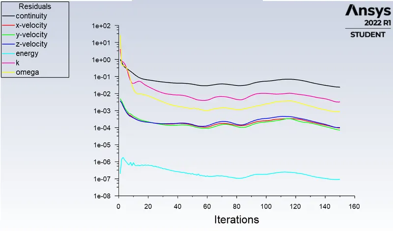
Result: we use 150 iterations to calculate the result.

Residual plot:

Temperature Contour plot:

Temperature plot in XY plane :

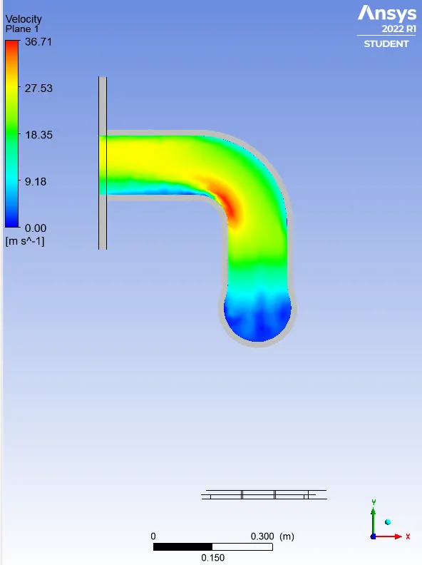
Velocity plot in XY plane :

Surface Heat Transfer Coefficient in XY plane :

Result Table:

Sr No Mesh Type No of Elements inflation layer Surface Heat Transfer Coeff.

1 Baseline Mesh 138132 Nil 22.5418

2 Refined Mesh 338040 8 22.3901

Analytical solution:

The Reynolds no. of the flow is Re=58168 considering the flow velocity =5 m/sec, D=Diameter of pipe=0.1699m

We use Dittus boelter equation for circular pipe

`N_u=0.023R_e^(0.8)*P_r^(n)` `rarr (1)`

Where n=0.4 for fluid being heated, `R_e`= Reynolds Number , `P_r`=Prandtl number

Prandtl number is given by ,

`P_r=(mu*C_p)/K` Here `mu` = 1.789 x`10^-5` Cp=1006.43 J/kgK , K=0.0242 W/mk

putting all these value in equation we get `P_r`=0.744

Put Re and Pr value in Equation (1) then `N_u`= 132.46

Nusselt Number = hL/K here L= Diameter of pipe hence `N_u`=hD/K

h= Nu*K/D hence by putting all the known value we get h=18.86 `W/(m^2*K)`

Conclusions:

• Heat transfer coefficient value from simulation is 22.54 and 22.39 and from analytical solution we get 18.86 that value is slightely close to the simulation result.
• Factors Affecting on prediction results is Elements size and quality,inflation layer,mesh at solid and fluid interface ie mesh at solid and fluid interface should be conformal.
• To verify the heat transfer coefficient of simulation result we required experimental data results for validation.
• The velocity at outlet is high because there are four inlets and one outlet so all the fluid will try to escape so the velocity get increased in that region.