Week 8- Moving zones approach in Fluent

Aim: To simulate rotary motion for the given geometry and to study the moving zones approach in Fluent.

Introduction:

• Introduction to moving zone :

Two types of motion are involved in the fluid flow problem

• Rectilinear
• Rotary.

To model Rotary motion, two approaches are used :

• Moving reference frame.
• Moving mesh approach

1. Moving Reference Frame (MRF):

The Moving Reference Frame Approach is a steady-state method employed in industrial Computational Fluid Dynamics to model problems with rotating parts.

• Types of Moving Reference Frame :

1. Single MRF: Refer to the entire computational domain to a Single moving reference frame approach
2. Multiple MRF: In complex geometry, it is not possible to use a single reference frame. In such cases break up the problem into multiple cell zones with well-defined interfaces between the cell zones.

In Ansys Fluent, by enabling the moving reference frame in selected cell zones, we can model the problem involving moving parts. when the moving reference frame is activated, equations of motion are modified by incorporating the additional acceleration term due to the transformation stationary reference frame to a moving reference frame. By solving these equations in a steady-state manner, the flow around the moving parts can be modeled.

Circular Kind of Interface:

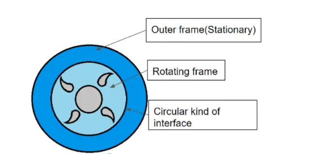
Fig: Circular Interface

• The Navier-stoke equation in a stationary frame is solved separately
• The Navier-stoke equation in the rotating frame is solved separately, as well
• Data is transferred from one frame to another frame through the interface
• Methods through which data is transferred through the interface

• Area averaging : Averaging the result at the interface over the area with this formula:

`phi=1/AintphidA`

• Mass averaging :

`phi_m=1/m intrho V phidA`

• Mixed-out approach :

Solves the following equations :

• Continuity
• X- momentum
• Y- momentum
• Z-momentum
• Energy

2.Moving Mesh Approach :

Used for modeling unsteady phenomena such as

• Vortex induced flows
• Interaction of vortex with bodies

• Sliding Mesh Approach : If unsteady interaction between stationary and moving parts is important then employ the sliding mesh method to capture the transient behaviour of the fluid flow.

Difference between Moving Reference Frame and Moving Mesh Approach

Sr No Moving Reference Frame Moving Mesh Approach

1 Frame is moving Mesh is moving

2 Mesh Topology remains same Topology changes with time

3 No change in control volume Control volume changes with time

4 Steady phenomenon Unsteady phenomenon

• Set Up :
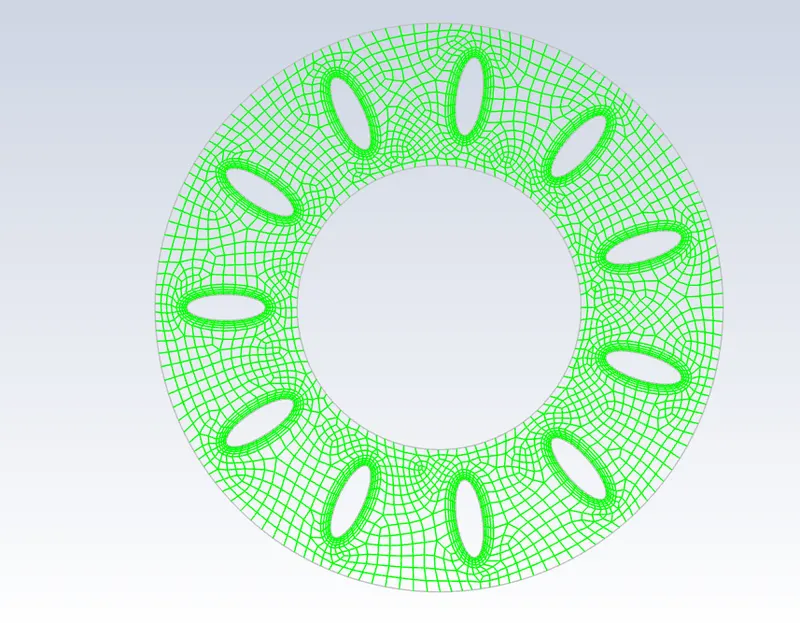
• Import the mesh file of the model into the set up :

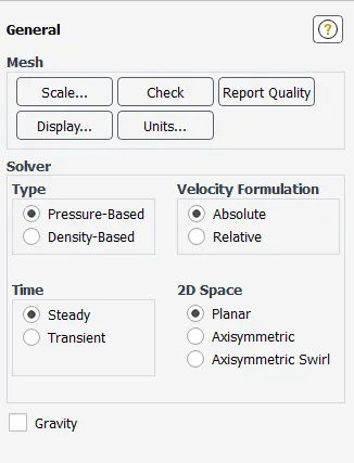
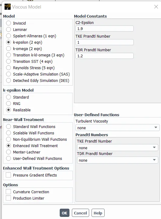
• Viscous Model :

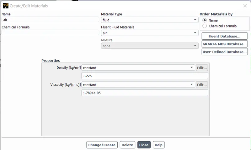
• Material :

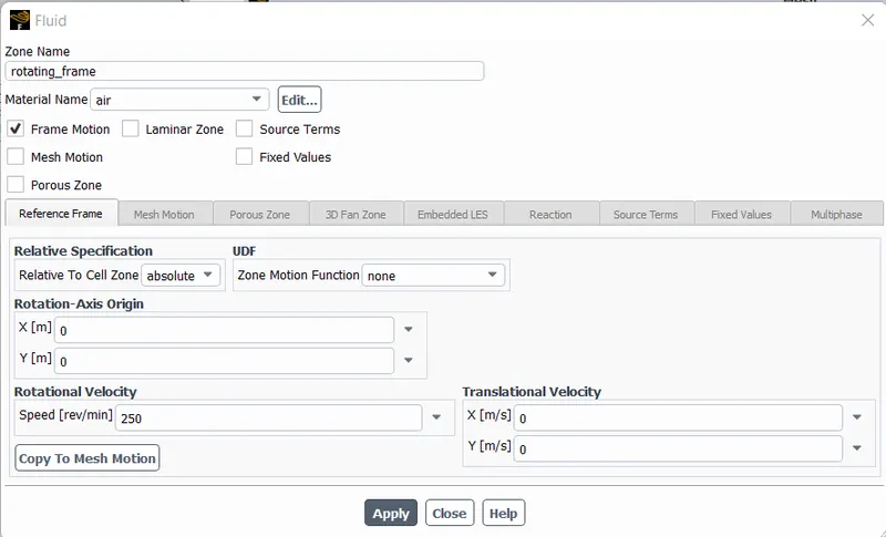
• Cell Zone Conditions :

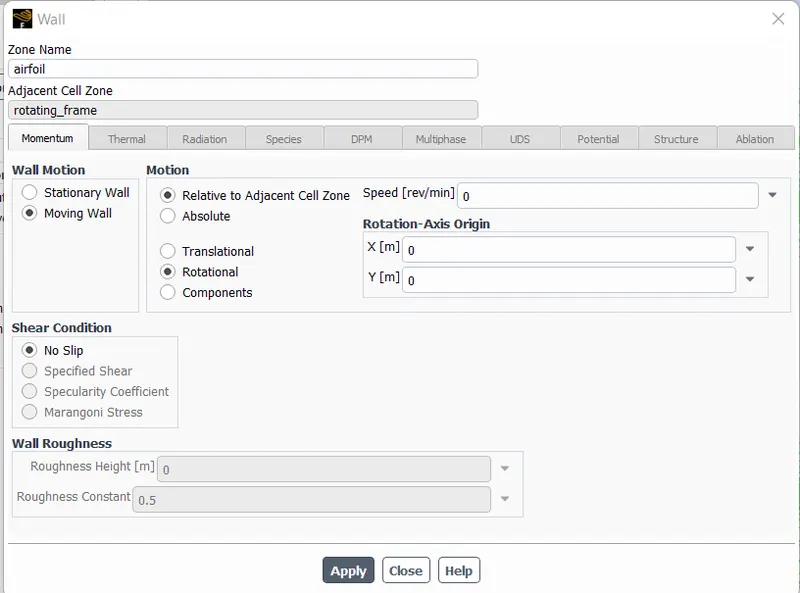
• Boundary Condition :

For aerofoil, Select a wall motion as Moving Wall and we check the motion is selected as Relative to Adjacent cell zone and Rotational.

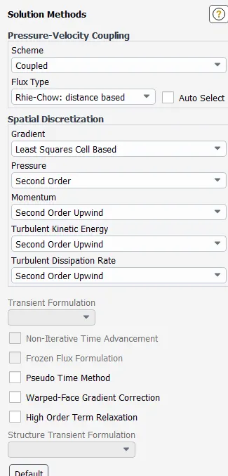
• Solution :

The solution scheme is set to Coupled and the spatial discretization is set to second-order upwind.

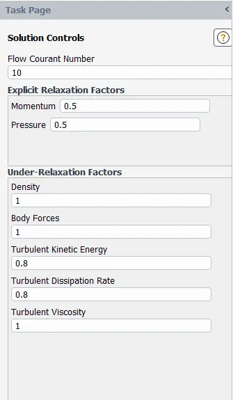
• Initialization :Hybrid Initialization :

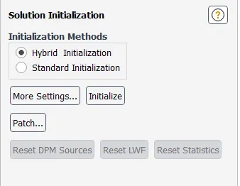
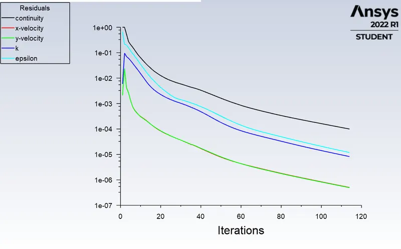
Run the simulation for 1000 iterations:

The solution is converged at 114 iterations.

• Results :
• Residual Plot:

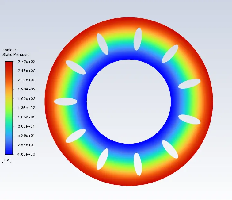
• Pressure Contour:

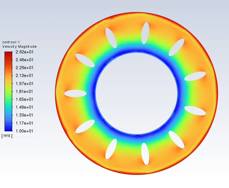
• Velocity Contour:

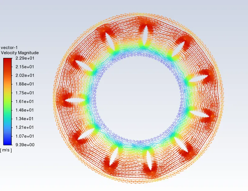
• Velocity Vector Plot:

• Conclusions:
• From the pressure contour, we observed that the pressure is negative at the inner side of the rotating domain where the suction of air takes place near the centre of impeller. and the pressure is maximum at the outer side of the rotating domain. and at the leading edge of the airfoil.
• The velocity is maximum (26.2m/sec) at the rotating domain outer and minimum (10m/sec) at the rotating domain inner .
• The velocity separation is observed at the Top edge of the airfoil,and velocity at Trailing edge of the aerfoil is also minimum.