Week 3 - Solving second order ODEs

Aim: To write the program to solve the ode which represent the equation of motion of simple pendulum with damping and also simulate the pendulum motion .

Procedure:

The equation of motion of a simple pendulum with damping

`(d^2theta)/dt^2+(b/m)(d theta)/(dt)+(g/L)sin theta=0`

Assume `theta=theta1=y(1)`

`(d theta)/dt=(d theta1)/(dt)=y(2)`

hence `(d theta2)/(dt)=(d^2theta1)/dt^2`by putting all this values and solving this equation we get two first order ODE

ydot(1)=y(2)

ydot(2)=-(b/m)*y(2)-(g/L)*sin(y(1))

Given parameters,

m=1kg

L=1 meter.

b=0.05

g=9.81 `m/(sec^2)`

time= 0 to 20 sec

Initial Condition :

Angular Displacement=0 at t=0 sec

Angular Velocity =3 rad/sec at t=0 sec

Matlab code for Defining Two function ydot(1) and ydot(2):

function[ydot]=odefun_simplependulum(t,y)
m=1;
l=1;
b=0.05;
g=9.81;
ydot=zeros(2,1);
ydot(1)=y(2);
ydot(2)=-(b/m)*y(2)-(g/l)*sin(y(1));
end

Explanation of above code is follows;

Step1) Define the function ydot

Step 2) Define all given parameter values ie m,g,b,l

Step 3) Generate the matrix of two rows and one column to store output values of ydot

Step 4)By entering the ydot(1) and ydot(2) function then end the function.

Final Matlab code

clear all
close all
clc
t=[0 20];
y0=[0 3];
% ode function 
[t,y]=ode45('odefun_simplependulum',t,y0);
%plotting graph
figure(1)
title('Angular Displacement vs time')
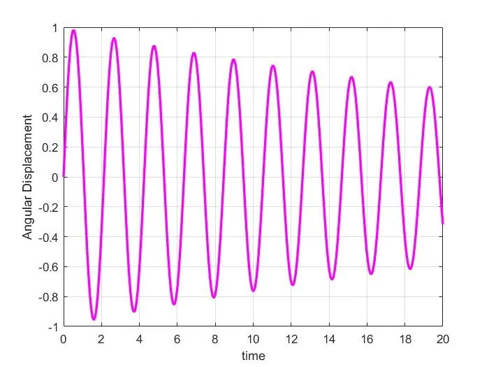
plot(t,y(:,1),'color','m','linewidth',2)
xlabel('time')
ylabel('Angular Displacement')

figure(2)
title('Angular Velocity vs time')
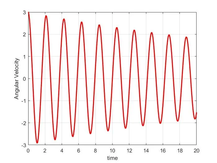
plot(t,y(:,2),'color','r','linewidth',2)
xlabel('time')
ylabel('Angular Velocity')
% Animation of motion
figure(3)
xlim([-1 1]);
ylim([-1.2 0]);
x0=0;
y0=0;
l=1;
for i=1:length(t)
    x1=l*sin(y(i,1));
    y1=-l*cos(y(i,1));
    grid on;
    string=line([x0,x1],[y0,y1]);
    center=[x1 y1];
    pendulum=viscircles(center,0.1)
    f(i)=getframe(gcf);
    delete(string);
    delete(pendulum);
end
    myvideo=VideoWriter('Pendulum.avi');
    open(myvideo)
    writeVideo(myvideo,f);
    close(myvideo);

Explanation Of above code :

Step 1) Represent the time value which is given in equation 0 to 20sec

Step 2) The initial condition ie Angular Displacement=0 at t=0 sec,Angular Velocity =3 rad/sec at t=0 sec ie y(0)=[0 3]

Step 3) Represent the ODE45 function and call the function from external function ie odefun_simplependulum, time span and initial condition.

Step 4) Plotting the graph of angular displacement vs Time by using plot command,and is represent in figure (1)

Step 5) Plotting the graph of angular Velocity vs Time by using plot command,and is represent in figure (2)

Step 6) For the Animation in video format we use x limit and y limit for display of output in that region

Step 7) Put x0=0,y0=0, for the fixed point of pendulum and given length l=1m .

Step 8) By using the for loop we create the image of simple pendulum for given value of time as 0 to 20sec

and x1 y1 is the location of simple pendulum at angular dispacement for the different value of a time .

Step 9) String command is used to connect the line from the (x0 y0) and(x1 y1)

we use getframe command to capture current figures

Step 10) By using the VideoWriter command we represent the motion of a simple pendulum in figure(3)

Result:

1) The graph of angular displacement vs time : Figure(1)

2) The graph of angular Velocity vs time: Figure (2)

3) The simulation of simple pendulum motion ie figure(3) ie AVI file is attached with this answer.