Week 8 - Simulating Cyclone separator with Discrete Phase Modelling

Aim:- To perform analysis on cyclone separator and calculate the separation efficiency and pressure drop.

Objective:-

1. To write a few words about any four empirical models used to calculate the cyclone separator efficiency.
2. To perform an analysis on a given cyclone separator model by varying the particle diameter from 1 μm to 5 μm and calculate the separation efficiency in each case. Discuss the results. [Use both the velocity's as 3m/sec.]
3. To perform an analysis on a given cyclone separator model by varying the particle velocity from 1 m/sec to 5 m/sec and calculate the separation efficiency and pressure drop in each case. Discuss the results. [Use particle diameter size as 5 μm for all cases & keep flow velocity same as particle velocity]

Procedure:

Introduction :

Cyclone separator are a low-cost, low-maintenance way of separating particulate matter from air or other gas streams. This separator is mainly used for the separation of solids from liquids. It mainly consists of a tangential inlet to feed the materials inside the chamber. It has solid and fluid outlets which separate fluid through one side and solids through the other side.

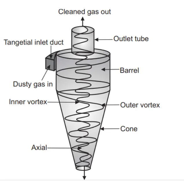
Working of Cyclone separator:

Typically, air is supplied tangentially at a very high velocity into solid-gas suspensions to cause rotating movement within the vessel. The fluid (gas) is drained from the top’s central outlet. The particles are acted on by centrifugal force due to the cyclone separator’s rotatory flow. Solids are hurled against the walls, generating an outer vortex, before falling to the conical base and being released through the solids outlet. The particles are separated from the air stream by centrifugal force caused by the increased air velocity in the outer vortex. When air reaches the bottom of the cone, it starts to flow radially inwards and out at the top as clean air/gas, while particulates fall into the cyclone’s dust collection chamber.

The efficiency of cyclone collection varies depending on density, particle size, and cyclone design. Increases in particle size and/or density, intake duct velocity, cyclone body length, number of gas revolutions in the cyclone, ratio of cyclone body diameter to gas exit diameter, inlet dust loading, smoothness of the cyclone inner wall, and other factors all contribute to cyclone efficiency. Similarly, as characteristics such as gas viscosity, cyclone body diameter, gas exit diameter, gas inlet duct area, gas density, and air leakage into the dust outlet grow, cyclone efficiency may drop.

Applications :

1. Cyclone separator is used to separate the suspensions of a solid in a gas or air.
2. To remove coal dust in power plant .
3. Used as spray dryer or gasification reactor.
4. It can be used in air-handling systems to produce particle-free clean air.

four empirical models used to calculate the cyclone separator efficiency :

1) lozia and Leith model:

Iozia and Leith model is modified version of Barth model. This model is developed based upon force balance. The model assumes that a particle carried by the vortex endures the influence of two forces i.e. centrifugal force and flow resistance.

Collection efficiency of a particles with diameter`d_("pi")`can be calculated as-

`eta_i=1/(1+(d_(pc)/d_("pi"))^beta)`

Where,

`beta="Expression for slope parameter"`

`beta=0.62-0.87ln(d_(pc)/100)+5.21ln((ab)/D^2)+1.05ln((ab)/D)^2`

`d_(pc)="50% cut size"`

`d_(pc)=[(9muQ)/(pirho_pz_cv_(tmax)^2)]^0.5`

2) Li and Wang model:

Li and Wang model includes particle bounce or re-entrainment and turbulent diffusion at cyclone wall. A two dimensional analytical expression of particle distribution in cyclone is obtained.

This model based on following assumption-

• The radial particle velocity and the radial concentration profile are not constant for uncollected particles within the cyclone.
• Boundary conditions with the consideration of turbulent diffusion coefficient and particle bounce re-entrainment on the cyclone wall are:

`c=c_0" at "theta=0`

`D_r(delc)/(delr)=(1-alpha)omegac" at "r=D/2`

• The tangential velocity is related to the radius of cyclone by:`uR^n = "constant"`

The collection efficiency can be formulate as-

`eta_i=1-exp{-lambdatheta_1}`

where,

`theta_1=2pi(S+L)/a`

`lambda=((1-alpha)komega_w)/(D_rr_w^n)`

3. Koch and Licht model:

Koch and Licht collection theory recognized the inherently turbulent nature of cyclones and the distribution of gas residence times within the cyclone. Koch and Licht described particle motion in the entry and collection regions with the additional following assumptions:

• The tangential velocity of a particle is equal to the tangential velocity of the gas flow, i.e. there is no slip in the tangential direction between the particle and the gas.
• The tangential velocity is related to the radius of cyclone by: `uR^n = "constant"`

The efficiency can be calculated as-

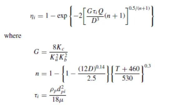
Here G is the factor related to configuration of cyclone and n is related to vortex and `tau`is the relaxation term

4. Lapple model:

Lapple model was developed based on force balance without considering the flow resistance. Lapple assumed that a particle entering the cyclone is evenly distributed across the inlet opening. The particle that travels from inlet half width to the wall in the cyclone is collected with 50% efficiency.

The semi empirical relationship developed by Lapple to calculate a 50% cut diameter, dpc, is

`d_(pc)=[(9mub)/(2piN_ev_i(rho_p-rho_g))]^0.5`

Where,

`N_e = "Number of revolution"`

`N_e=1/a[(H+h)/2]`

And efficiency can be given as

`eta_i=1/(1+(d_(pc)/d_("pi"))^2)`

Step 1) Geometry:

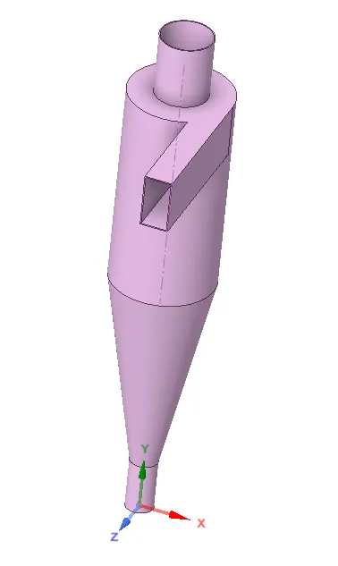
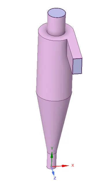
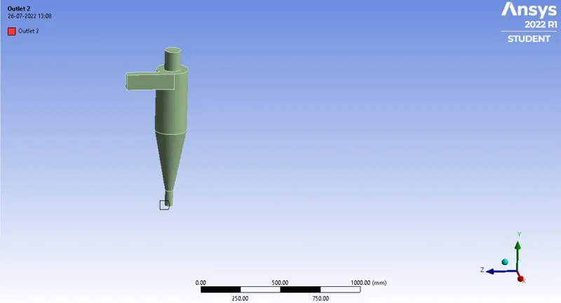
• The step file of cyclone separator was imported into the spaceclaim
• Go to prepare option and select the volume extract and select the edges of the inlet and outlet (top) and outlet (bottom)
• After obtaining the fluid volume, the remaining geometry is suppressed for physics,since the fluid will not be present in this region .
• The next step is to mesh the fluid volume.

Step 2) Mesh:

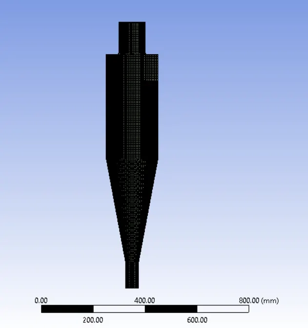
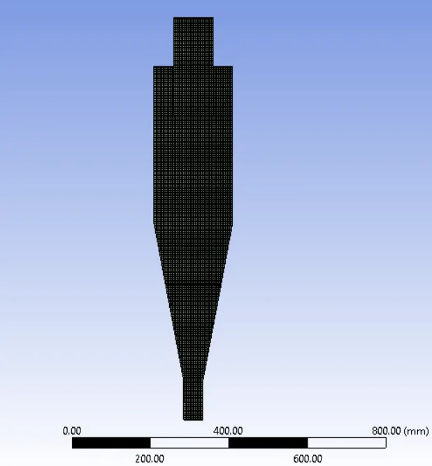
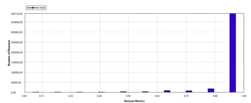
• In this case the flow is swirling and we have to track the particles and obtain the particle history data ,it is important to have equally size mesh elements within the geometry.
• Hence we use cartesian method to get equal volume of mesh elements in the geometry
• We use global element size is 10mm and cartesian mesh size is set to 5 mm
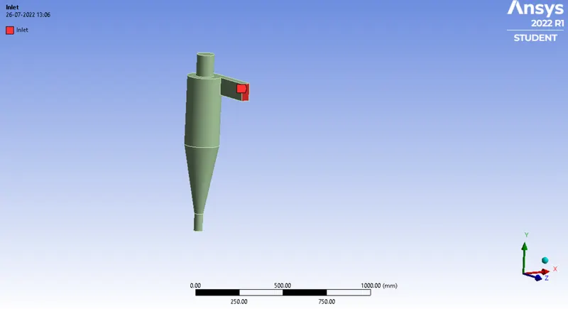
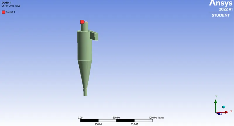
• By using named selection we give appropriate name to boundaries.

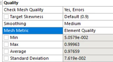
Elemental Quality:

Step 3) Set up and solution:

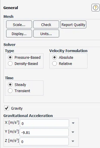
• In this case we use pressure based solver and we select steady state .
• We enabled the gravity and put value 9.81 `m/sec^2` -ve Y direction.
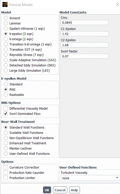
• The K-epsilon RNG model was used in this particular problem.
• The swirl dominated flow option turned on for this simulation.
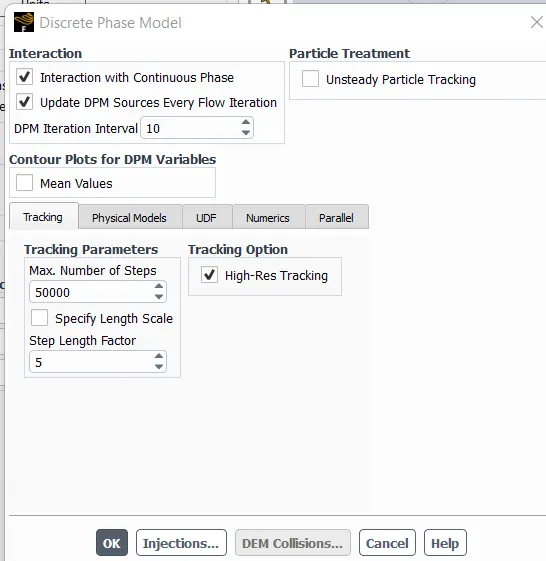
• After that discrete phase model is turned and settings are changed.
• We turned on interaction with continuous phase which enable a coupled flow.and also enable Update DPM sources every flow iteration .
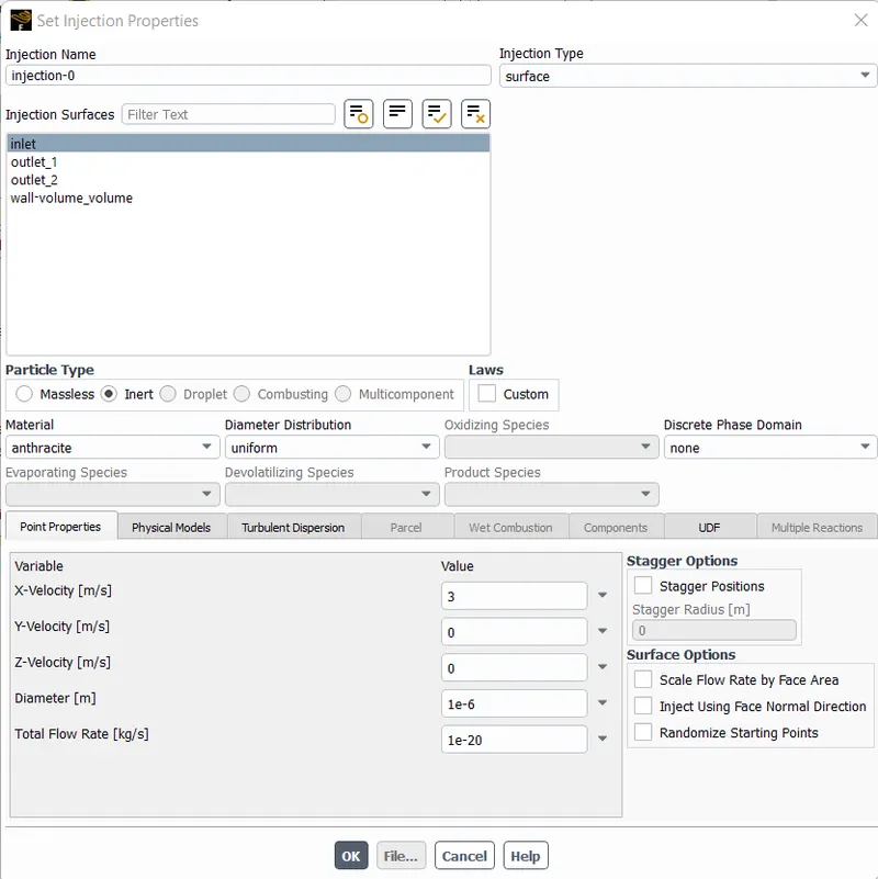
• The new injection was created with the following parameters :M
• Material : anthracite
• Particle type:Inert
• Diameter distribution : uniform
• Injection type- surface
• Release from - inlet
• Velocity - 1,3,5 m/sec in x direction
• Diameter of particle -1,3,5 microns
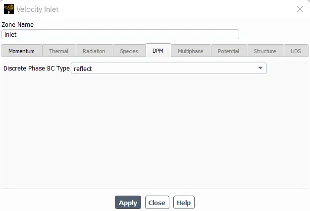
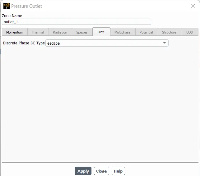
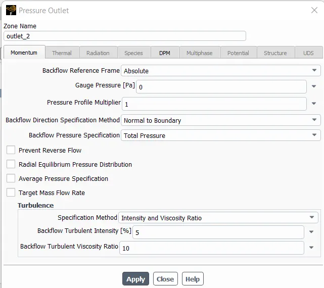
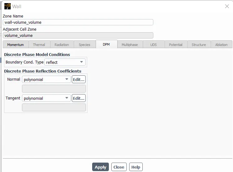
• The boundary condition for DPM were set accordingly
• Inlet- Reflect
• wall- Reflect
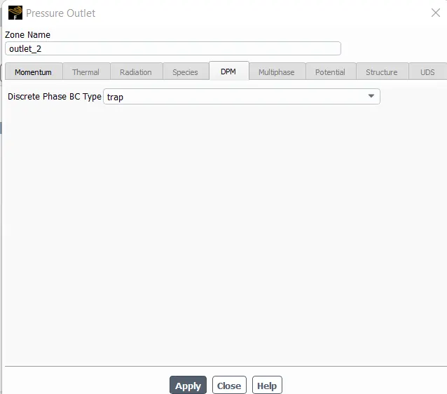
• Outlet (Top)-escape
• Outlet(Bottom)-trap
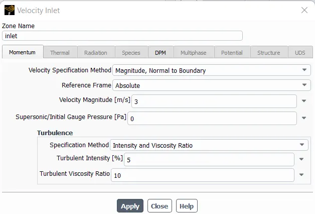
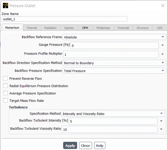
• The inlet is a velocity inlet and outlet is a pressure outlet.
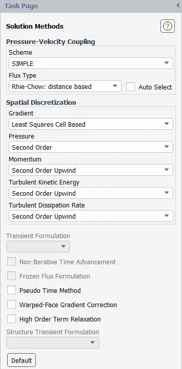
• Solution method is Simple and select second order upwind Turbulent kinetic energy and turbulent dissipation rate .
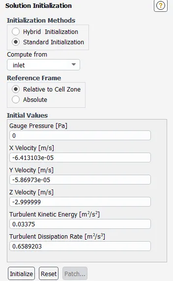
• The solution was initialised using standard initialisation and was computed from inlet.
• The problem was then run for 800 iterations and the results were observed

Step 4) Results :

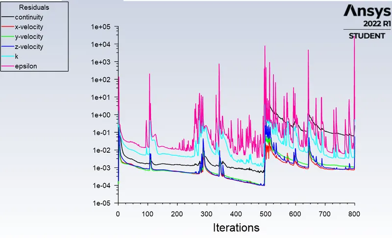
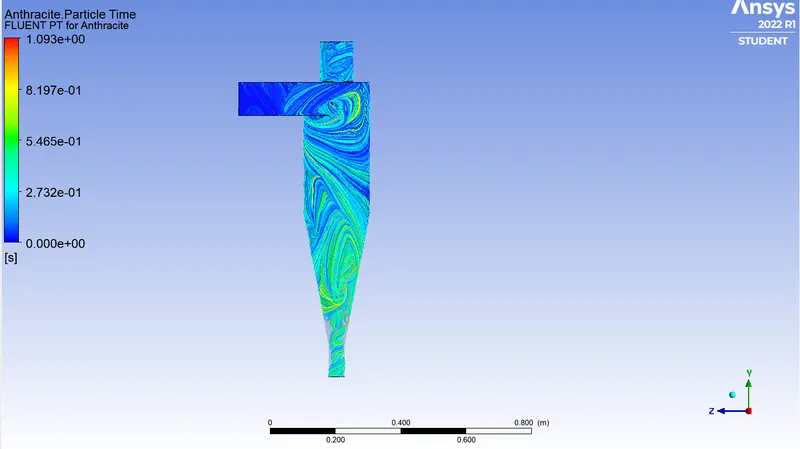
Case 1)Velocity :3 m/sec Particle Diameter size :`1e^-6` m

Residual plot:

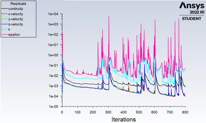
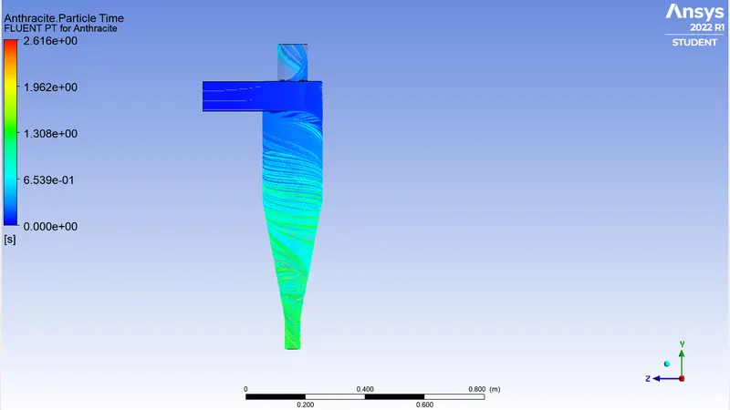
Case 1) Velocity :3 m/sec Particle Diameter size : `3e^-6` m

Residual plot:

Case 1) Velocity :3 m/sec Particle Diameter size : `5e^-6` m

Residual plot:

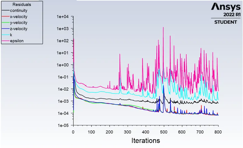
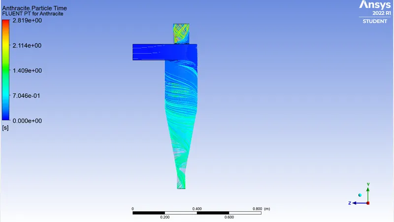
Case 2) Velocity :1 m/sec Particle Diameter size : `5e^-6`m

Residual plot:

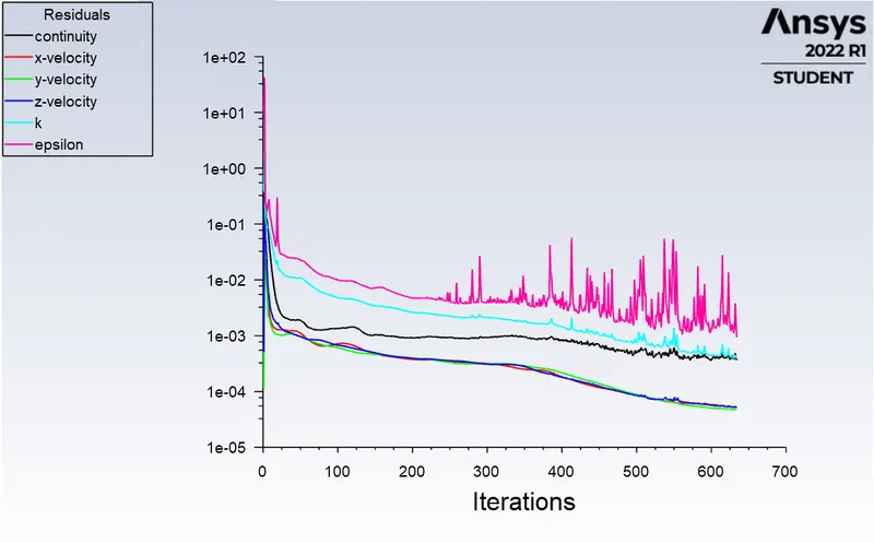
Solution is converged at 634 iterations.

Pressure Drop plot:

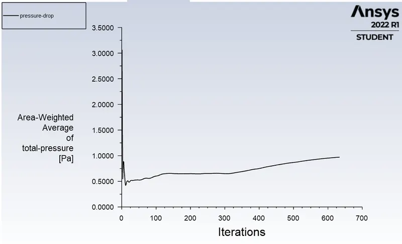
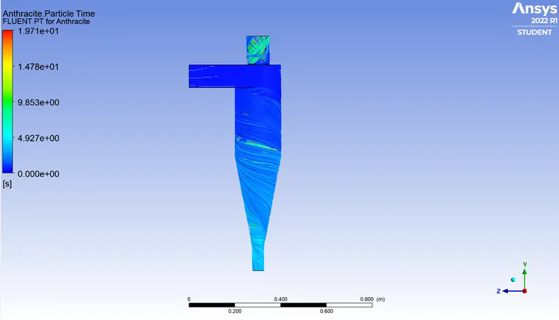
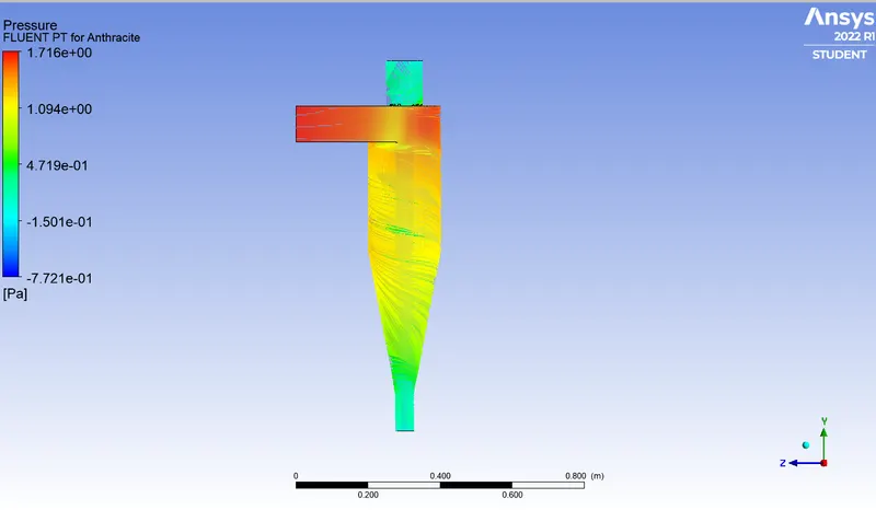
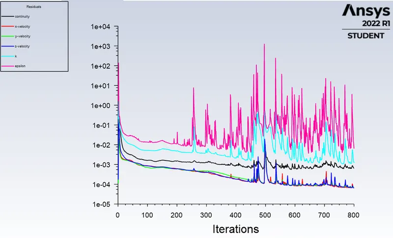
Case 2) Velocity :3 m/sec Particle Diameter size : `5e^-6`m

Residual plot:

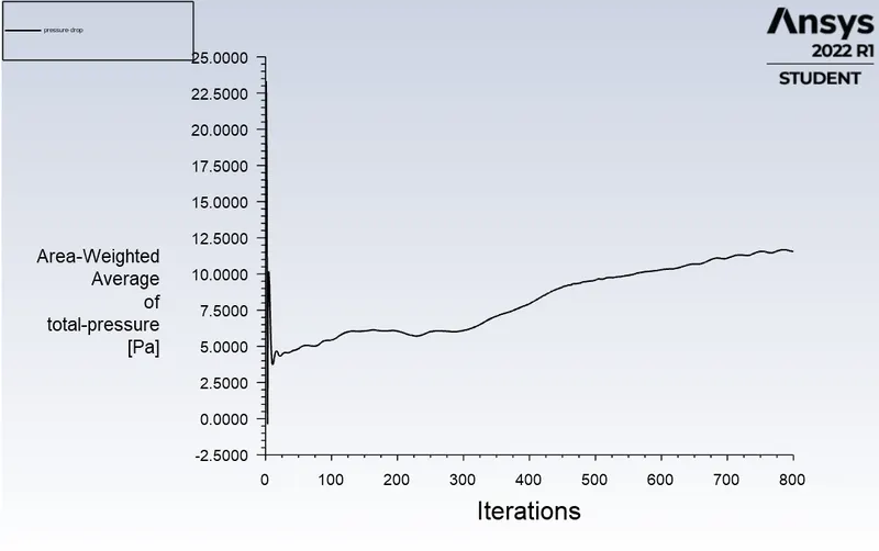
Pressure Drop plot:

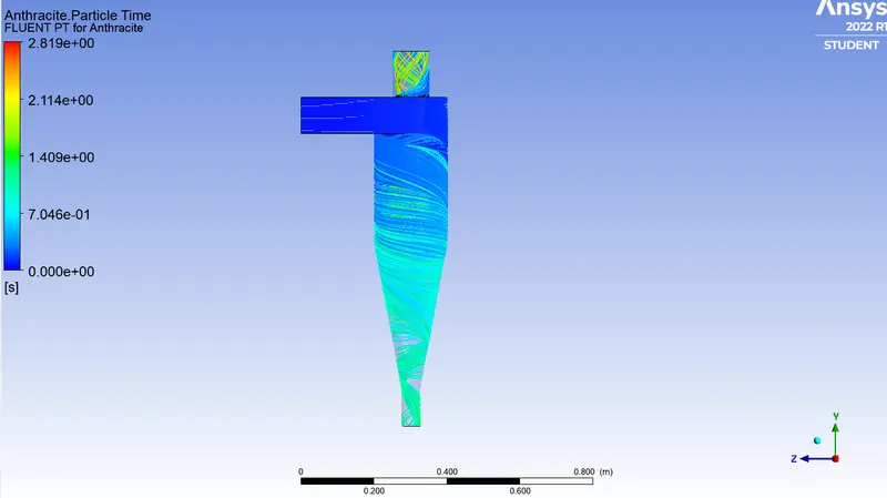
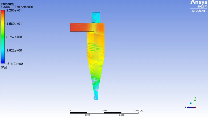
Case 2) Velocity :5 m/sec Particle Diameter size :`5e^-6`m

Residual Plot:

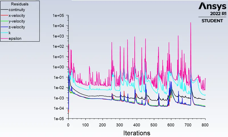
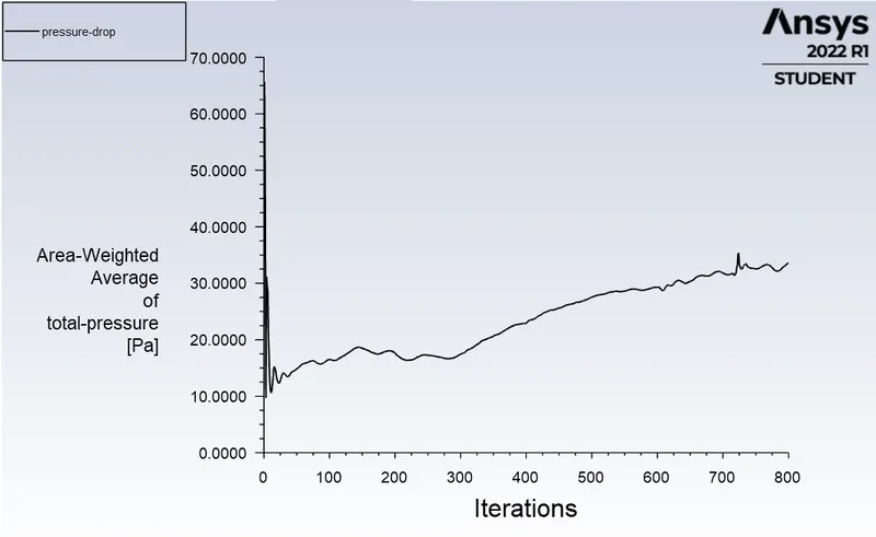
Pressure Drop plot:

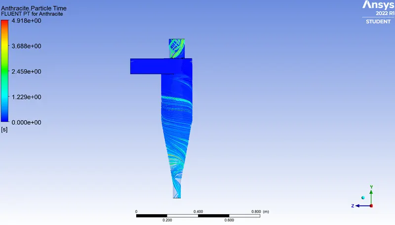
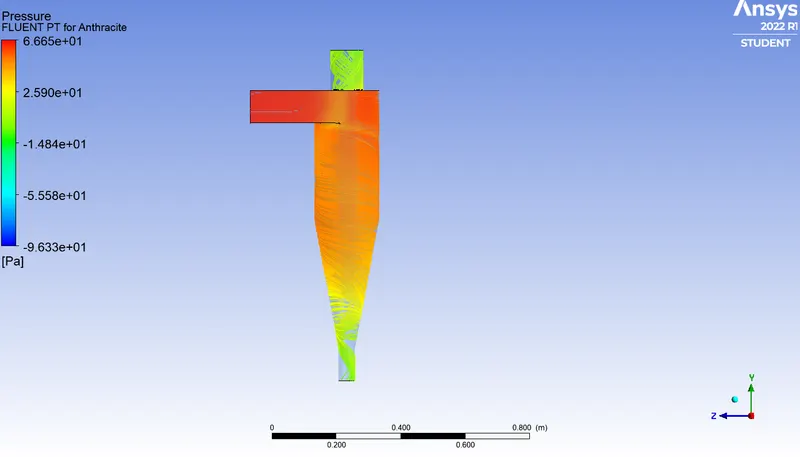
Case 1) Results are tabulated as follows:

Sr No	Particle Size (micron)	Particle velocity (m/sec)	Particle Tracked	Particle Escaped	Particle Trapped	Incomplete	Separation efficiency (%)
1	1	3	378	178	193	7	51.05
2	3	3	378	45	333	0	88.09
3	5	3	378	102	276	0	73.01

Case 2) Results are tabulated as follows:

Sr No	Particle Size (micron)	Particle velocity (m/sec)	Particle Tracked	Particle Escaped	Particle Trapped	Incomplete	Separation efficiency (%)	Pressure Drop (Pa)
1	5	1	378	96	282	0	74.6	0.97
2	5	3	378	102	276	0	73.01	11.56
3	5	5	378	106	272	0	71.95	33.56

Conclusions:

• The separation efficiency is increasing if we increase the particle size with constant particle velocity and flow velocity.
• The pressure drop is increases if we increase the particle velocity.
• With increase in velocity at a constant particle size the separation efficiency is slightly decreases.