Week 8 - Simulation of a backward facing step in OpenFOAM

Aim:

• To simulate an incompressible-laminar-viscous flow through the backward facing step geometry.
• Perform a transient simulation. The solver can be chosen based on the described physics of the flow.
• Explain the simulation process and also provide explanations to every change you make inside the reference case files obtained from OpenFOAM tutorials.
• Perform 2 case studies as described below and compare the results.
• 1)Case 1: Simulate the flow without using any grading factor (i.e., GF = 1)
• 2)Case 2: Simulate the flow with grading factor of 0.2. The cells should be finer near the walls (includig the step wall).

Procedure:

• Open the Openfoam tutorial and find the solver to solve incompressible-laminar-viscous flow problem.
• After finding the solver next step is to copy the file in to the OpenFOAM run folder so that the official file of the openfoam remains unchanged.
• Find out blockMesh Dict script file to create the given geometry and provide mesh specification.
• Find controlDict file to edit start and end time for simulation.
• In the folder '0' we can set initial parameter for velocity and pressure according to the faces of the given domain.
• Use blockMesh command to generate the mesh.
• Open the simulation file in paraview and plot the velocity profile at point 0.085m from inlet.
• Repeat the above procedure for grading factor 0.2 to check the differences in the results.

Problem Statement:

Simulate an incompressible-laminar-viscous flow through the backward facing step geometry.

Perform 2 case studies as described below and compare the results.

Case 1 - Simulate the flow without using any grading factor (i.e., GF = 1)

Case 2 - Simulate the flow with grading factor of 0.2. The cells should be finer near the walls (includig the step wall).

Mesh specification

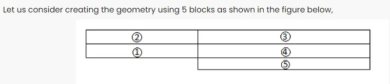
1. Number of cells along the x direction (longer dimension) = 200
2. Number of cells along the longer y direction = 20;

Boundary condition specification

The domain specifications are provided in the following figure.

The following steps is used to simulate the given problem:

Case 1 - Simulate the flow without using any grading factor (i.e., GF = 1)

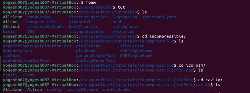
Step 1) first use Ctrl+Alt+T to open the new terminal then type foam to open the openfoam and then type tut to find the appropriate tutorial to solve the given problem .use ls command ie ls means list,to view the list in that folder

Step 2) Our problem is incompressible-laminar-viscous flow problem. so we can change the directory by using cd command and choose the incompressible file and in that file choose icofoam solver because in order to solve the navier stokes equation for the incompressible laminar flow problem.

Step 3)In that icofoam we select the cavity folder to create the required domain.

Step 4) To copy the file in to the OpenFOAM run folder we use cp command and create the copy of cavity as Cavity_test1,and check the file created and open that file Cavity_test1, lets check the directories present in the Cavity_test1 file by using ls command.

Step 5) Open the system folder by using cd command and view the list of directories using ls command , we use the gedit command to edit the content of any script file ,1st we edit the blockMeshDict file to create the domain and provide the required specification for block mesh.

Step 6) We do the following changes to generate block mesh

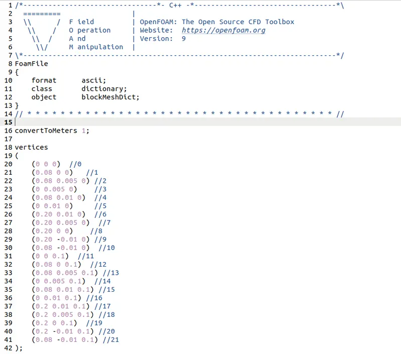
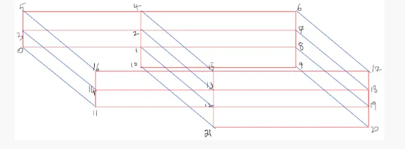
Step 7)To create the geometry 1st we have to add the vertices total 21 vertices are used to create the geometry.

The 21 vertices which is used to create the geometry is shown in fig below and the values of co-ordinates such as x,y,z are used as per given domine specification but for the thickness of the block we assume the z value is 0.1

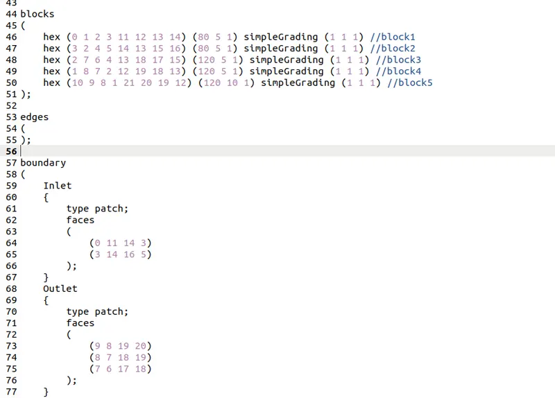
The next step is to define the types of mesh here we use the hexahedral mesh.Let us consider the line no 46

hex (0 1 2 3 11 12 13 14) (80 5 1) simpleGrading (1 1 1) //block1 here we use hex (8 vertices) and then next bracket contain the mesh points along the x,y,z direction of the block which represent as (nx,ny,nz) in order to obtain the uniform mesh points for given domain we change the nx, ny value accordingly. nz=1 because this is 2D problem and last one is simlpeGrading this is for streching the mesh points as per our requirements and application along x,y,z direction of block similarly we use this technique for block2,block3,block4,block5 .

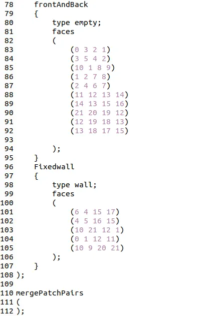
Step 8) The next step is to define the boundary conditions we define the conditions as per given conditions.

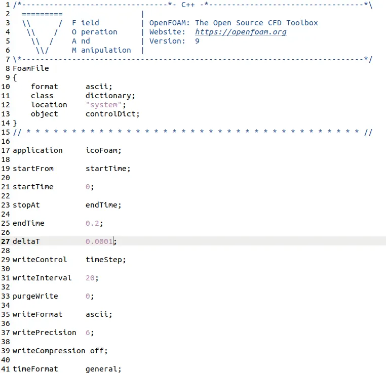
Step 9)To set the start and end time for simulation we use gedit command and edit the controlDict script file and set the end time is 0.2 and delta T=0.0001.

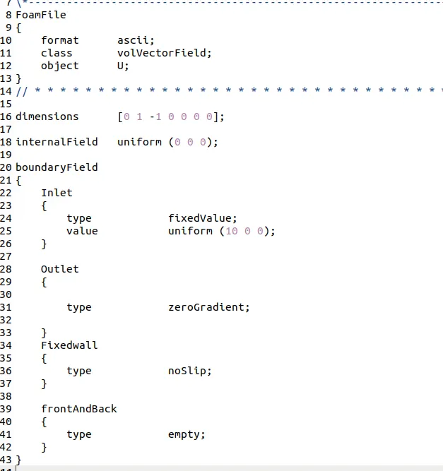
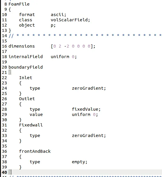
Step 10) To set the initial boundary condition for pressure and velocity at each faces and also update the name of boundary same as we updated in blockMeshDict. for laminar flow we use velocity along x direction is 10m/sec for simulation.The required changes in p and U script file is as follows: for velocity :

for pressure:

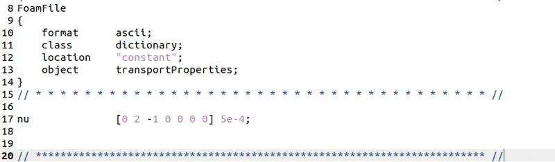
we also required to enter the value of kinematic viscosity hence for that we use the procedure below :

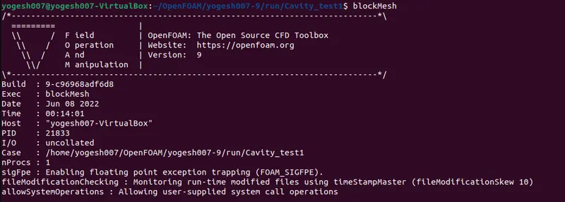
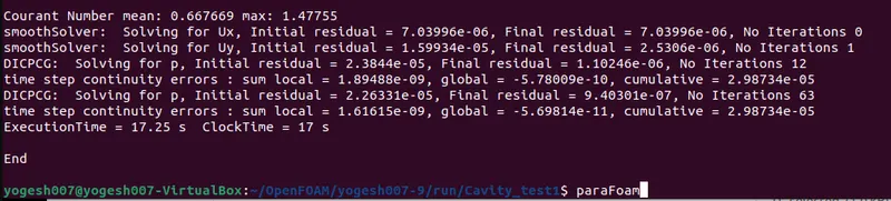
we check the block mesh by using blockMesh commad and then we use the icoFoam solver command directly to run the simulation

and after that we use paraFoam command to view the geometry and mesh .

The given geometry with uniform mesh points are shown in figure below :(case 1)

Result:

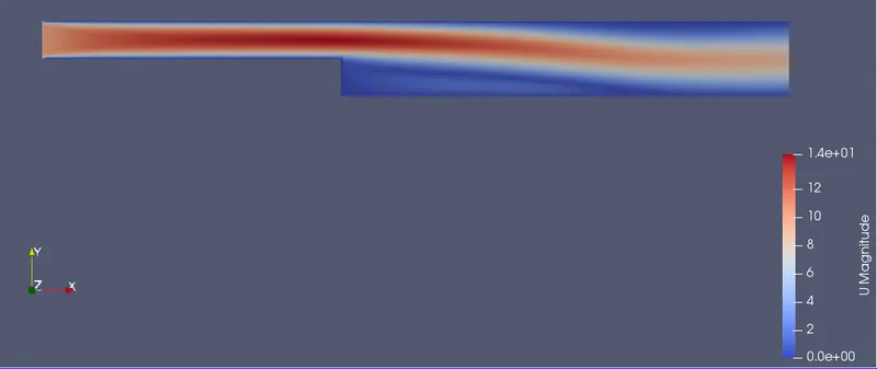
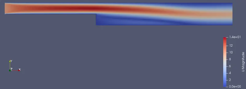
• Velocity Distribution over domine area : for case 1 (Grading factor is 1)

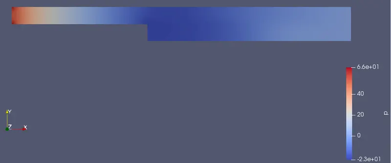
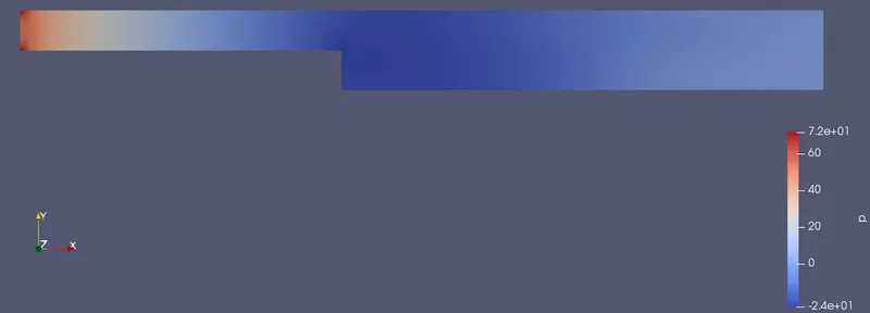
• Pressure Distribution over domine area : for case 1 (Grading factor is 1)

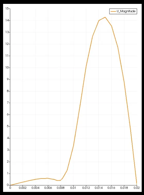
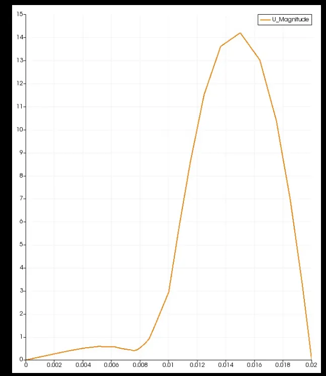
• Velocity profile at 0.085 m from the inlet of the geometry : for case 1 (Grading factor is 1)

For the simulation of case 2 all the process is same but we have to make the changes in blockMeshDict script file which is shown in figure below:

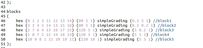
Mesh grid for case 2 (Grading factor is 0.2)

• Velocity Distribution over domine area : for case 2 (Grading factor is 0.2)

• Pressure Distribution over domine area : for case 2 (Grading factor is 0.2)

• Velocity profile at 0.085 m from the inlet of the geometry : for case 2 (Grading factor is 0.2)

Conclusion:

• Grading factor and their Importance in meshing :

1) In computational fluid dynamics the grading is useful for computational efficiency. In CFD fluid always shows the largest changes in near the walls or obstacles so in order to capture that changes we always use fine mesh near the wall.

2) To get the effective and reliable results. we have to know where to use fine grading factor . so for obtaining the more effective results, if we use large number of fine elements in mesh,It could increases the computational time for converging the solution but it is helpful to capture the flow at boundary walls and obstacles.

• By comparing the results obtained from both the cases we conclude that the results obtained are approximately same but the execution time for case 2 is slightly higher than case 1 .