Week 5 - Turbulence modelling challenge

Objectives:

1. In this challenge, you are required to do a literature review of various turbulence models explained in the Turbulence modeling video (Week-5) and explain why DNS isn’t feasible according to Kolmogorov's scale.
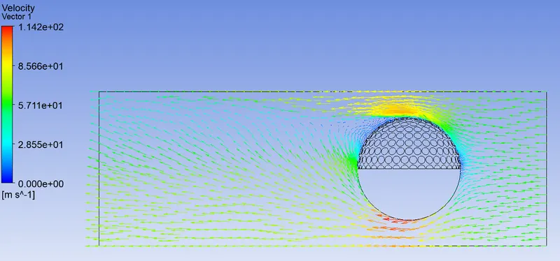
2. For the below geometry performs a 3D simulation and explain the recirculation region using velocity vectors.
3. Consider the flow direction of air, the ball is traveling opposite to it at 60m/s. Explain in which direction the ball will curve by visualizing the wake region.

Introduction :

The kind of flow is determined by the Reynolds Number :

Reynolds Number :

The ratio of inertia force to viscous force is called as Reynolds number.

1. Laminar flow :

• Occur at low Reynolds number
• Viscous forces are dominant
• Characterized by smooth ,constant fluid motion.

2.Turbulent flow:

• Occurs at high Reynolds number
• Inertia forces are dominant .
• Produce chaotic eddies ,vortices and other instabilities

3.Transition flow :

• Energy and momentum transfer are strongly influenced by either inertial or non linear effects that are unique to the simulation .

According to the order of PDEs the Turbulent models are classified into two types

1. First order model
2. Second order model

1. First order model : Assumes an analogy between laminar and turbulent flows ,Average turbulent flow field is similar to corresponding laminar flow .Uses first order PDEs to solve for turbulent viscosity.

First order models:

• Zero equation model
• One equation model (Spalart Allmaras model)
• Two equation model: 1. k-`epsilon` model, 2.k-`omega` model
• Zero equation model : The zero equation model does not employ PDEs to account for turbulent viscosity
• One equation model (Spalart Allmaras model):

PDE is used for solving turbulent kinetic energy to obtain turbulent viscosity

Turbulent .

Turbulent Kinetic energy is determined from

K=`1/2(bar(u^2)+bar(v^2)+bar(w^2))`

Turbulent viscosity is determined by,

`mu_t`=C`sqrt(Kl_m`

Turbulent viscosity is substituted in RANS

The Spalart Allmaras model is designed especially for internal flow and external aerodynamic applications.

Especially when flow is attached.Not good for flow with strong adverse gradient

• Two equation model: Two PDE are used to solve for

1.Turbulent Kinetic energy and Turbulent dissipation rate

2.Turbulent Kinetic energy and Specific dissipation rate

Most commonly used method in industries.

• k`-epsilon` Model :The K-epsilon model is good for turbulent flows with no flow separation.

1.Standard k `epsilon`model: Most widely used model for industrial applications.Uses wall functions for calculating `epsilon` near walls . Known to have very good convegence and memory efficient.Good for attached and turbulent flow.Good in solving external flow around complex bodies.Performs poorly for separated flow.

2.Realizable k -`epsilon`model: Modify the `epsilon` equation .Solve some of constraints on Reynolds stresses .Shows consistent results with physics of turbulent flow.

3.Renormalized Group ( RNG) k-`epsilon` model: Improved `epsilon` equation.Effect of swirl is introduced .It uses empirical relations to find a modified version of Prandtl Number.

• k -`omega` model :The k-omega model is most widely utilized in industry.This model does not contain terms undefined at the wall Wall function is not required at the wall.

1.Standard k-`omega` model: Most widely adopted in aerospace and turbomachinery components.

2.SST k-`omega`model : Shear stress transfer k-omega model .It is a better variant of the traditional k-`omega` model.Uses a blending function to transition from standard model to a higher Reynolds model away from the wall.

• Second order Model: Solves transport equations for Reynolds stress term .For 3D additional equations needs to be solved .Most accurate result.computationally expensive.This model is highly sensitive to Boundary conditions.

1.Algebraic stress model

2.Reynolds stress model

According to Kolmogorov's scale.DNS isn’t feasible.

Ans : Solve NS equations at a very small scales

According to Kolmogrov scale,

`eta`= `1/(Re^(3/4)`

• Grid size must be smaller than this .
• In 3D Each dimension of the element must be smaller than the length determined from kolmogrov scale.

Volume= `1/(Re^(9/4)`

Number of elements = `V/(DeltaV)`

where, V=Structural overall volume

`DeltaV`= Volume of smallest elements

Number of elements `prop` `Re^(9/4)`

• This leads to a very large number of elements in 3D
• So DNS is still performed in 2D
• Using this method for industrial application is next to impossible.

Procedure:

Step 1) Import the geometry :

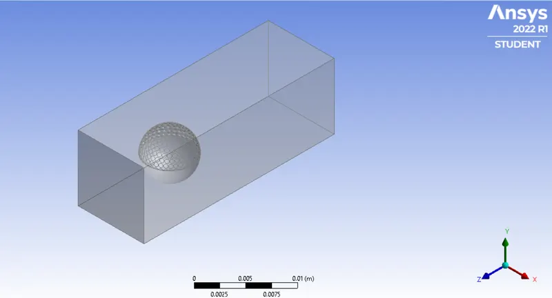
The given geometry is symmetric along YZ plane .

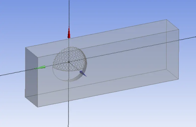
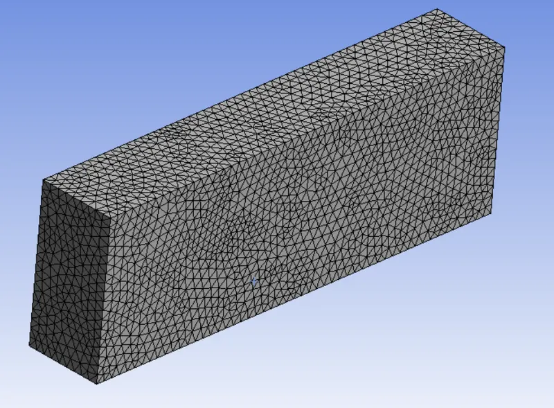
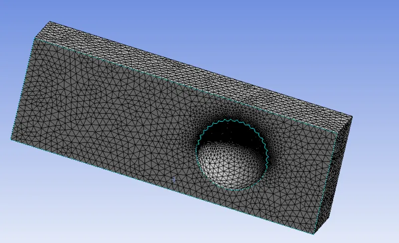
Step 2) Mesh :

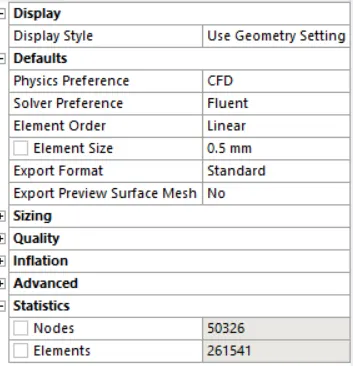
Step 3)Set up and solution:

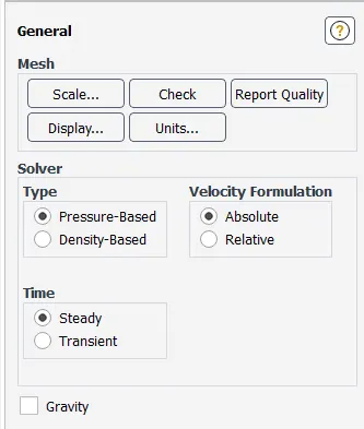
Material : Air

Velocity : 60 m/sec

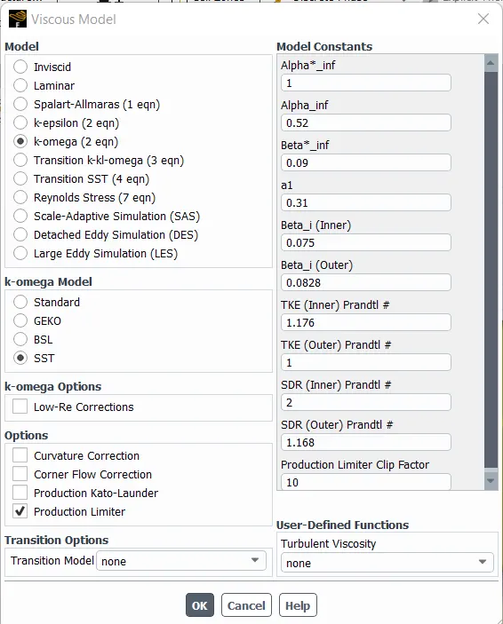
Viscous Model:

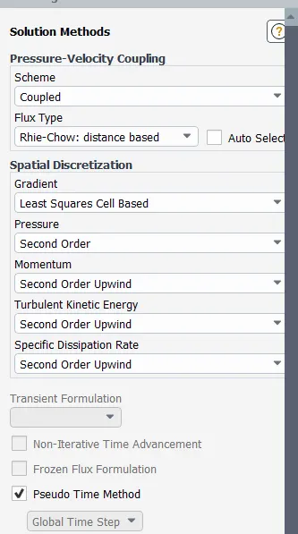
Solution method :

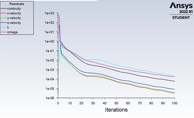
No of iterations : 100

Residual Plot :

Results :

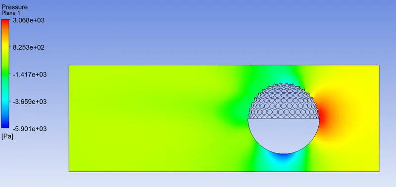
Pressure contour:

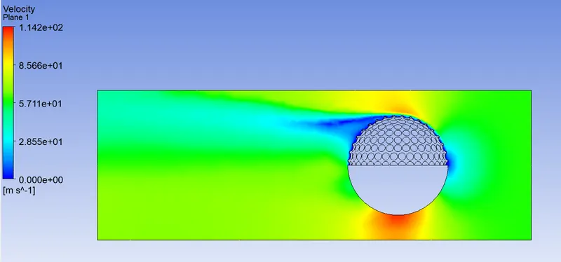
Velocity contour:

Velocity vector plot :

Conclusions:

• Simulation on golf ball is done using Ansys fluent.
• We can see from the velocity vector contour that the recirculations region is found behind the golf ball and that will tends to move the golf ball towards downward direction .The velocity of air at rough side of the golf ball is lower and at smooth side of golf ball is higher and this causes a pressure difference and due to that golf ball will move downward direction
• The dimples provided at top side of golf ball it will minimize the pressure drag and also minimize the recirculations region (wake region) .