Week 7 - Simulation of a 1D Super-sonic nozzle flow simulation using Macormack Method

Aim:To simulate the isentropic flow through a quasi 1D subsonic-supersonic nozzle for both the conservation and non-conservation forms of the governing equations and solve them using the MacCormack's technique.

Procedure:

1D super-sonic nozzle flow:

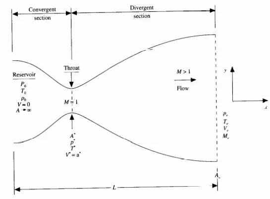
We consider the steady, isentropic flow through a convergent-divergent nozzle which is shown in figure(a)

Figure(a)

We are using book for reference computational fluid dynamics by John D Anderson .The flow at the inlet to the nozzle comes from the reservoir where the pressure and temperature are denoted by `p_0 and T_0` respectively.The cross sectional area of the reservoir is large( A tends to infinity) and hence the velocity is very small(V→0)Thus the `p_0 and T_0` are the stagnation values or total pressure and total temperature respectively. The flow expands isentropically to supersonic speeds at the nozzle exit,where the exit pressure,temperature,velocity and mach number are denoted by Pe,Te,Ve,Me

respectively.The flow is locally subsonic in the convergent section of the nozzle,sonic at the throat(minimum area) and supersonic at the divergent section.The sonic flow(M=1)at the throat means that the local velocity at this location is equal to the local speed of the sound.using an asterisk to denotes the sonic flow values ,we have at the throat `V=V^ast=a^ast`.Similarly the sonic flow values of pressure and temperature are denoted by `P^ast and T^ast`respectively.The area of the sonic throat is denoted by `A^ast` We assume that at a given section, where the cross-sectional area is A,the flow properties are uniform across that section.Hence, although the area of the nozzle changes as a function of distance along the nozzle, x, and therefore in reality the flow field is two-dimensional (the flow varies inthe two dimensional xy space.we make the assumption that the flow properties vary only with x; this is tantamount to assuming uniform flow properties across any given cross section .such flow is defined as quasi one dimensional flow.

The governing continuity,momentum and energy equations for this quasi one dimensional steady,isentropic flow can be expressed ,respectively as,

continuity Equation `rho_1*V_1*A_1=rho_2*V_2*A_2`

Momentum Equation `P_1A_1+rho_1V_1^2A_1+int_(A_1)^(A_2) PdA=P_2A_2+rho_2V_2^2A_2`

Energy Equation `h_1+V_1^2/2=h_2+V_2^2/2`

Generally ,governing equations are two types conservative and non conservative form.Here we are solving both the forms ,

Conservative form:

Continuity Equation `(del(rhoA))/(delt)+(del(rhoAV))/(delx)=0`

Momentum Equation: `(del(rhoAV))/(delt)+(del[rhoAV^2+(1/gamma)*(P*A)])/dx`=`(1/gamma)*(P)*(delA)/(delx)`

Energy equation : `(del[rho(e/(gamma-1)+gamma/2*V^2).A])/(delt)+(del[rho(e/(gamma-1)+gamma/2*V^2)A.V+PAV])/(delx)=0`

Non Conservative form:

Continuity Equation: `(delrho)/(delt)=-rho(delV)/(delx)-rho*V*(del(lnA))/(delx)-V*(delrho)/(delx)`

Momentum Equation: `(delV)/(delt)=-V(delV)/(delx)-1/(gamma)((delT)/(delx)+T/rho(delrho)/(delx))`

Energy Equation: `(delT)/(delt)=-V(delT)/(delx)-(gamma-1)T((delV)/(delx)+V(del(lnA))/(delx))`

MacCormack method:

MacCormack method is a widely used discretization scheme for the numerical solution of hyperbolic partial differential equations.The Maccormack method is a variation of the two steps Lax wrendroff scheme but is much simpler in the application .It is second order accurate in both space and time .For second order accuracy in time a predictor- corrector strategy is used and their average is employed to calculate the actual derivatives.In the predictor step the governing equation is replaced spatial derivative by using forward differences and in corrected step with backward differencing.

Non- Conservative form:

Predicted step:

Forward differencing

`((delrho)/(delt))_i^t=-rho_i^t*(V_(i+1)^t-V_i^t)/(Deltax)-rho_i^t*V_i^t(lnA_(i+1)-lnA_i)/(Deltax)-V_i^t(rho_(i+1)^t-rho_i^t)/(Deltax)`

`((delV)/(delt))_i^t=-V_i^t*(V_(i+1)^t-V_i^t)/(Deltax)-1/gamma((T_(i+1)^t-T_i^t)/(Deltax)+T_i^t/rho_i^t*(rho_(i+1)^t-rho_i^t)/(Deltax))`

`((delT)/(delt))_i^t=-V_i^t*(T_(i+1)^t-T_i^t)/(Deltax)-(gamma-1)*(T_i^t)((V_(i+1)^t-V_i^t)/(Deltax)+V_i^t(lnA_(i+1)-lnA_i)/(Deltax))`

We obtain the updated values of `rho , T , V`using the above predicted values

`rho_i^(t+Deltat)=rho_i^t+((delrho)/(delt))_i^t*Deltat`

`V_i^(t+Deltat)=V_i^t+((delV)/(delt))_i^t*Deltat`

`T_i^(t+Deltat)=T_i^t+((delT)/(delt))_i^t*Deltat`

Corrected step:

Backward Differencing

`((delrho)/(delt))_i^(t+Deltat)=-rho_i^(t+Deltat)*(V_(i)^(t+Deltat)-V_(i-1)^(t+Deltat))/(Deltax)-rho_i^(t+Deltat)*V_i^(t+Deltat)(lnA_(i)-lnA_(i-1))/(Deltax)-V_i^(t+Deltat)(rho_(i)^(t+Deltat)-rho_(i-1)^(t+Deltat))/(Deltax)`

`((delV)/(delt))_i^(t+Deltat)=-V_i^(t+Deltat)*(V_(i)^(t+Deltat)-V_(i-1)^(t+Deltat))/(Deltax)-1/gamma((T_(i)^(t+Deltat)-T_(i-1)^(t+Deltat))/(Deltax)+T_i^(t+Deltat)/rho_i^(t+Deltat)*(rho_(i)^(t+Deltat)-rho_(i-1)^(t+Deltat))/(Deltax))`

`((delT)/(delt))_i^(t+Deltat)=-V_i^(t+Deltat)*(T_(i)^(t+Deltat)-T_(i-1)^(t+Deltat))/(Deltax)-(gamma-1)T_(i)^(t+Deltat)((V_(i)^(t+Deltat)-V_(i-1)^(t+Deltat))/(Deltax)+V_(i)^(t+Deltat)*(lnA_(i)-lnA_(i-1))/(Deltax))`

The average time derivative are taken by ,

`((delrho)/(delt))_(avg)=0.5[((delrho)/(delt))_i^t+((delrho)/(delt))_i^(t+Deltat)]`

`((delV)/(delt))_(avg)=0.5[((delV)/(delt))_i^t+((delV)/(delt))_i^(t+Deltat)]`

`((delT)/(delt))_(avg)=0.5[((delT)/(delt))_i^t+((delT)/(delt))_i^(t+Deltat)]`

finally we calculate the `rho,V,T`values for the next time step `(t+Deltat)`

`rho_i^(t+Deltat)=rho_i^t+((delrho)/(delt))_(avg)*Deltat`

`V_i^(t+Deltat)=V_i^t+((delV)/(delt))_(avg)*Deltat`

`T_i^(t+Deltat)=T_i^t+((delT)/(delt))_(avg)*Deltat`

From the Anderson text book the shape of the nozzle is given by

Area `A=1+2.22*(x-1.5)^2` `0<=x<=3`

Boundary Conditions:

The initial conditions are specified as

`rho=1-0.3146x`

`T=1-0.2314x`

`V=(0.1+1.09x)*T^(1/2)`

Boundary condition at subsonic inflow is

`V(1)=2*V(2)-V(3)`

Boundary condition at supersonic outflow

`rho(n)=2.rho(n-1)-rho(n-2)`

`V(n)=2.V(n-1)-V(n-2)`

`T(n)=2.T(n-1)-T(n-2)`

Conservative form:

Lets us define the elements of solution vector (U),Flux vector (F) and source term (J) as follows,

`U_1=rho^' A^'`

`U_2=rho^'A^'V^'`

`U_3=rho^'(e^'/(gamma-1)+(gamma)/(2)*V^('2))A^'`

`F_1=rho^'A^'V^'`

`F_2=rho^'A^'V^('2)+(1/gamma*P'*A')`

`F_3=U_3V'+P'*A'*V'`

`J_2=1/gamma*P'*(delA')/(delx')`

With these elements the governing equations can be written as ,

`(delU_1)/(delt')=(delF_1)/(delx')`

`(delU_2)/(delt')=-(delF_2)/(delx')+J_2`

`(delU_3)/(delt')=-(delF_3)/(delx')`

To obtain the primitive variables we have to decode the elements `U_1,U_2,U_3` as follows

`rho^'=U_1/A^'`

`V'=U_2/U_1`

`T^'=e^'=(gamma-1)(U_3/U_1-gamma/2*V^('2))`

`P=rho^'*T^'`

Pure form of the flux terms

`F_1=U_2`

`F_2=U_2^2/U_1+(gamma-1)/gamma(U_3-gamma/2*U_2^2/U_1)`

`F_3=gamma*(U_2U_3)/U_1-gamma*(gamma-1)/2*U_2^3/U_1^2`

`J_2=(gamma-1)/gamma(U_3-gamma/2*U_2^2/U_1^2)(del(lnA))/(delx`

As similar to non conservative form In the predicted step the governing equation is replaced spatial derivatives by forward differences and in the corrected step with backward differencing.then take the average of them and update the final solution.

Initial conditions:

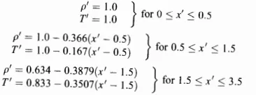
Since the dependent variables being solved U1, U2, U3 we need initial conditions for these same variables at time t=0 in order to start the finite difference solution . The initial conditions for U1,U2,U3 are allowed initial conditions for F1,F2,F3 to be obtained. such initial conditions for F1,F2 and F3 are needed to form the x derivatives on the right hand side.

The initial conditions are

Boundary conditions :

The boundary conditions for the subsonic-supersonic isentropic flow solution using the conservative form of the governing equations are theoretically the same .

The flow properties at the downstream,supersonic outflow boundary are obtained by linear extrapolation from the two adjacent internal points.If n denotes the grid points at the outflow boundary then

`(U_1)_n=2(U_1)_(n-1)-(U_1)_(n-2)`

`(U_2)_n=2(U_2)_(n-1)-(U_2)_(n-2)`

`(U_3)_n=2(U_3)_(n-1)-(U_3)_(n-2)`

Main Matlab code:

clear all
close all
clc
% Defining the inputs
%length of the nozzle
L=3;
%No of grid points
n=31;
%Defining mesh
x=linspace(0,L,n);
%mesh size 
dx=x(2)-x(1);
%Throat
throat=(n+1)/2;
% Number of time steps
nt=1400;
%Area
a=1+2.2.*(x-1.5).^2;
% Fluid properties
gamma=1.4;
C=0.5;  %CFL number

% Non conservative form
[rho_Nc,V_Nc,T_Nc,P_Nc,M_Nc,Mass_flow_Nc]=Non_con(n,x,dx,gamma,throat,nt,a,C);

% Conservative form
[rho_c,V_c,T_c,P_c,M_c,Mass_flow_c]=Conser(n,x,dx,gamma,throat,nt,a,C);

%Comparison of steady state result conservative and non conservative form
%(Non dimensional)
Terms=[{'Density'};{'Temperature'};{'Velocity'};{'Pressure'};{'Mach no'}];
Exact_sol=[0.634;0.833;1;0.528;1];
Non_conservative_sol=[rho_Nc(throat);T_Nc(throat);V_Nc(throat);P_Nc(throat);M_Nc(throat)];
Conservative_solution=[rho_c(throat);T_c(throat);V_c(throat);P_c(throat);M_c(throat)];
table(Terms,Exact_sol,Non_conservative_sol,Conservative_solution)

%Comparison of Normalizing mass flow rate distributions of Non conservative
%and conservative form
 figure(7)
 plot(x,Mass_flow_c)
 hold on
 plot(x,Mass_flow_Nc)
 xlabel('Length of nozzle')
 ylabel('Mass flow rate')
 legend('Conservative form','Non conservative form')
 title('Comparison of mass flow rate distributions of conservative and Non conservative form ')
grid on
warning("off")

Non Conservative form Function Code:

function [rho_Nc,V_Nc,T_Nc,P_Nc,M_Nc,Mass_flow_Nc]=Non_con(n,x,dx,gamma,throat,nt,a,C)

% calculate initial profiles 
rho_Nc=1-0.3146.*x;   %Density
T_Nc=1-0.2314.*x;     %Temperature
V_Nc=(0.1+1.09*x).*T_Nc.^0.5; %Velocity
% Non conservative form of supersonic nozzle flow equation
%Maccormack method
%outer loop

tic
for k=1:nt
    %create copy 
    rho_old=rho_Nc;
    V_old=V_Nc;
    T_old=T_Nc;
    dt=min(C.*dx./(sqrt(T_Nc)+V_Nc));
    %predicted step
    for i=2:n-1
        %derivatives
        dv_dx=(V_Nc(i+1)-V_Nc(i))/dx;
        drho_dx=(rho_Nc(i+1)-rho_Nc(i))/dx;
        dloga_dx=(log(a(i+1))-log(a(i)))/dx;
        dT_dx=(T_Nc(i+1)-T_Nc(i))/dx;

        %Continuity equation 
        drho_dt_p(i)=-rho_Nc(i)*dv_dx-rho_Nc(i)*V_Nc(i)*dloga_dx-V_Nc(i)*drho_dx;

        %Momentum equation
        dv_dt_p(i)=-V_Nc(i)*dv_dx-(1/gamma)*(dT_dx+(T_Nc(i))/(rho_Nc(i))*drho_dx);

        % Energy equation
        dT_dt_p(i)=-V_Nc(i)*dT_dx-(gamma-1)*T_Nc(i)*(dv_dx+V_Nc(i)*dloga_dx);

        %solution updates
        V_Nc(i)=V_Nc(i)+dv_dt_p(i)*dt;
        rho_Nc(i)=rho_Nc(i)+drho_dt_p(i)*dt;
        T_Nc(i)=T_Nc(i)+dT_dt_p(i)*dt;

    end
     
    % corrected step
    for i=2:n-1
         %derivatives
        dv_dx=(V_Nc(i)-V_Nc(i-1))/dx;
        drho_dx=(rho_Nc(i)-rho_Nc(i-1))/dx;
        dloga_dx=(log(a(i))-log(a(i-1)))/dx;
        dT_dx=(T_Nc(i)-T_Nc(i-1))/dx;

        %Continuity equation 
        drho_dt_c(i)=-rho_Nc(i)*dv_dx-rho_Nc(i)*V_Nc(i)*dloga_dx-V_Nc(i)*drho_dx;

        %Momentum equation
        dv_dt_c(i)=-V_Nc(i)*dv_dx-(1/gamma)*(dT_dx+(T_Nc(i))/(rho_Nc(i))*drho_dx);

        % Energy equation
        dT_dt_c(i)=-V_Nc(i)*dT_dx-(gamma-1)*T_Nc(i)*(dv_dx+V_Nc(i)*dloga_dx);

    end
    %compute the average time derivative
    drho_dt=0.5*(drho_dt_p+drho_dt_c);
    dv_dt= 0.5*(dv_dt_p+dv_dt_c);
    dT_dt=0.5*(dT_dt_p+dT_dt_c);

    % Final solution update
    for j=2:n-1
        rho_Nc(j)=rho_old(j)+drho_dt(j)*dt;
        V_Nc(j)=V_old(j)+dv_dt(j)*dt;
        T_Nc(j)=T_old(j)+dT_dt(j)*dt;
    end
    %Applying Boundary conditions
    %Inlet Boundary conditions
    V_Nc(1)=2*V_Nc(2)-V_Nc(3); %velocity 
    %outlet Boundary conditions
   V_Nc(n)=2*V_Nc(n-1)-V_Nc(n-2);
   rho_Nc(n)=2*rho_Nc(n-1)-rho_Nc(n-2);
   T_Nc(n)=2*T_Nc(n-1)-T_Nc(n-2);
       
   % Calculating pressure,Mach number and mass flow rate 
   P_Nc=rho_Nc.*T_Nc;         % Pressure
   M_Nc=V_Nc./(T_Nc.^(0.5));  %Mach number
   Mass_flow_Nc=rho_Nc.*a.*V_Nc; %Mass flow rate

   %Capturing primitive variable at throat for each time step 
   rho_throat(k)=rho_Nc(throat);
   V_throat(k)=V_Nc(throat);
   P_throat(k)=P_Nc(throat);
   T_throat(k)=T_Nc(throat);
   M_throat(k)=M_Nc(throat);
   flow_rate_throat(k)=Mass_flow_Nc(throat);

   figure(1)
   % Variation of Mass flow rate distribution inside the nozzle at
   % different time steps during the time marching process 
   if k==150
       plot(x,Mass_flow_Nc)
       hold on
   elseif k==250
           plot(x,Mass_flow_Nc)
           hold on
           elseif k==450
                  plot(x,Mass_flow_Nc)
                  hold on
           elseif k==900
                  plot(x,Mass_flow_Nc)
                  hold on
           elseif k==1200
                  plot(x,Mass_flow_Nc)
                  hold on
                  legend('@150','@250','@450','@900','@1200')
                  title('Mass flow rate distribution at different time steps in Non conservative form')
                 xlabel('Length of nozzle(Non dimensional)')
                 ylabel('Mass flow rate in Non conservative form ')
                 grid on
   end
end
Time_Nc=toc
figure(2)
% Time wise of the primitive variables amd mach number at the nozzle throat
% Time wise variation of the primitive variables
plot(M_throat)
hold on
plot(rho_throat)
hold on
plot(V_throat)
hold on
plot(T_throat)
hold on
plot(P_throat)
legend('Mach Number','Density(Non dimensional)','Velocity(Non dimensional)','Temperature(Non dimensional)','Pressure(Non dimensional)')
xlabel('No of time steps')
ylabel('Mach no,Density,Velocity,Temperature,Pressure')
title('Timewise variation of non dimensional primitive variables at throat in Non conservative form')
grid on
figure(3)
% Steady state distribution of primitive variables inside the nozzle
subplot(5,1,1)
plot(x,M_Nc)
xlabel('Length of nozzle(non dimensional)')
ylabel('Mach no')
title('Steady state distribution of primitive variables inside the nozzle in Non-conservative form')
subplot(5,1,2)
plot(x,V_Nc)
xlabel('Length of nozzle(non dimensional)')
ylabel('Velocity(Non dimensional)')
subplot(5,1,3)
plot(x,rho_Nc)
xlabel('Length of nozzle(non dimensional)')
ylabel('Density(ND)')
subplot(5,1,4)
plot(x,T_Nc)
xlabel('Length of nozzle(non dimensional)')
ylabel('Temperature(ND)')
subplot(5,1,5)
plot(x,P_Nc)
xlabel('Length of nozzle(non dimensional)')
ylabel('Pressure(ND)')
grid on
end

Conservative form Function code:

function [rho_c,V_c,T_c,P_c,M_c,Mass_flow_c]=Conser(n,x,dx,gamma,throat,nt,a,C);

% calculate initial profiles 
for i=1:n
    if x(i)<0.5
        rho_c(i)=1;
        T_c(i)=1;
    elseif x(i)>=0.5 && x(i)<1.5
        rho_c(i)=1-0.366*(x(i)-0.5);
        T_c(i)=1-0.167*(x(i)-0.5);
    elseif x(i)>=1.5 && x(i)<=3.5
        rho_c(i)=0.634-0.3879*(x(i)-1.5);
        T_c(i)=0.833-0.3507*(x(i)-1.5);
    end
    V_c(i)=0.59/(rho_c(i)*a(i));

end

% Conservative form of supersonic nozzle flow equation
% Maccormack method
%Outer loop 
U1=rho_c.*a;
U2=rho_c.*a.*V_c;
U3=U1.*(T_c/(gamma-1))+((gamma/2).*V_c.^2);
tic
for k=1:nt
    dt=0.0267; %Textbook value in anderson to verify results
   % dt=min(C.*dx./(sqrt(T_c)+V_c));
    % predicted step 
    %create a copy
    U1_old=U1;
    U2_old=U2;
    U3_old=U3;

    F1=U2;
    F2=U2.^2./U1+((gamma-1)/(gamma)).*(U3-(gamma/2)*U2.^2./U1);
    F3=gamma.*U2.*U3./U1-0.5*gamma*(gamma-1).*U2.^3./U1.^2;

    for i=2:n-1
        J2=(1/gamma)*rho_c(i)*T_c(i)*((a(i+1)-a(i))/dx);

        dU1dt_p(i)=-(F1(i+1)-F1(i))/dx;
        dU2dt_p(i)=-(F2(i+1)-F2(i))/dx+J2;
        dU3dt_p(i)=-(F3(i+1)-F3(i))/dx; 

        %Updated values 
        U1(i)=U1_old(i)+dU1dt_p(i)*dt;
        U2(i)=U2_old(i)+dU2dt_p(i)*dt;
        U3(i)=U3_old(i)+dU3dt_p(i)*dt;
    end
    %Update of flux variables for corrected step 
    F1=U2;
    F2=U2.^2./U1+((gamma-1)/(gamma)).*(U3-(gamma/2)*U2.^2./U1);
    F3=gamma.*U2.*U3./U1-0.5*gamma*(gamma-1).*U2.^3./U1.^2;
    rho_c=U1./a;
    T_c=(gamma-1).*(U3./U1-(gamma/2).*(U2./U1).^2);

    %Corrected  step
    for i=2:n-1
        J2=(1/gamma)*rho_c(i)*T_c(i)*((a(i)-a(i-1))/dx);

        dU1dt_c(i)=-(F1(i)-F1(i-1))/dx;
        dU2dt_c(i)=-(F2(i)-F2(i-1))/dx+J2;
        dU3dt_c(i)=-(F3(i)-F3(i-1))/dx; 
    end
    %Compute the average time derivative
    dU1_dt=0.5*(dU1dt_p+dU1dt_c);
    dU2_dt=0.5*(dU2dt_p+dU2dt_c);
    dU3_dt=0.5*(dU3dt_p+dU3dt_c);

    %final Solution update
    for j=2:n-1
        U1(j)=U1_old(j)+dU1_dt(j)*dt;
        U2(j)=U2_old(j)+dU2_dt(j)*dt;
        U3(j)=U3_old(j)+dU3_dt(j)*dt;
    end
    % Applying the Boundary conditions
    %Inlet
    U1(1)=a(1);
    U2(1)=2*U2(2)-U2(3);
    V_c=U2(1)/U1(1);
    U3(1)=U1(1)*(T_c(1)/(gamma-1)+(gamma/2)*V_c(1)^2);

    % Outlet
    U1(n)=2*U1(n-1)-U1(n-2);
    U2(n)=2*U2(n-1)-U2(n-2);
    U3(n)=2*U3(n-1)-U3(n-2);
     
    rho_c=U1./a;
    V_c=U2./U1;
    T_c=(gamma-1).*(U3./U1-(gamma/2).*(V_c).^2);
    P_c=rho_c.*T_c;
    M_c=V_c./sqrt(T_c);
    Mass_flow_c=rho_c.*a.*V_c;

    % Capturing flow field value at throat for each time step 
    rho_throat(k)=rho_c(throat);
    V_throat(k)=V_c(throat);
    T_throat(k)=T_c(throat);
    P_throat(k)=P_c(throat);
    M_throat(k)=M_c(throat);
    Mass_flow_rate_throat(k)=Mass_flow_c(throat);

    figure(4)
    % Variation of Mass flow rate distribution inside the nozzle at
    % different time steps during the time marching process 
    if k==150
       plot(x,Mass_flow_c)
       hold on
   elseif k==250
           plot(x,Mass_flow_c)
           hold on
           elseif k==450
                  plot(x,Mass_flow_c)
                  hold on
           elseif k==900
                  plot(x,Mass_flow_c)
                  hold on
           elseif k==1200
                  plot(x,Mass_flow_c)
                  hold on
                  legend('@150','@250','@450','@900','@1200','Analytical solution','Initial flow rate')
                  title('Mass flow rate distribution (Non dimensional) at different time steps in conservative form')
                 xlabel('Length of nozzle(Non dimensional)')
                 ylabel('Mass flow rate in conservative form ')
                 grid on

   end
end
Time_c=toc
figure(5)
% Time wise of the primitive variables amd mach number at the nozzle throat
plot(M_throat)
hold on
plot(rho_throat)
hold on
plot(V_throat)
hold on
plot(T_throat)
hold on
plot(P_throat)
legend('Mach Number','Density(Non dimensional)','Velocity(Non dimensional)','Temperature(Non dimensional)','Pressure(Non dimensional)')
xlabel('No of time steps')
ylabel('Mach no,Density,Velocity,Temperature,Pressure')
title('Timewise variation of non dimensional primitive variables at throat in conservative form')
grid on

figure(6)
% Steady state distribution of primitive variables inside the nozzle
subplot(5,1,1)
plot(x,M_c)
xlabel('Length of nozzle(non dimensional)')
ylabel('Mach no')
title('Steady state distribution of primitive variables inside the nozzle in conservative form')
subplot(5,1,2)
plot(x,V_c)
xlabel('Length of nozzle(non dimensional)')
ylabel('Velocity(ND)')
subplot(5,1,3)
plot(x,rho_c)
xlabel('Length of nozzle(non dimensional)')
ylabel('Density(ND)')
subplot(5,1,4)
plot(x,T_c)
xlabel('Length of nozzle(non dimensional)')
ylabel('Temperature(ND)')
subplot(5,1,5)
plot(x,P_c)
xlabel('Length of nozzle(non dimensional)')
ylabel('Pressure(ND)')
grid on

end

Results:

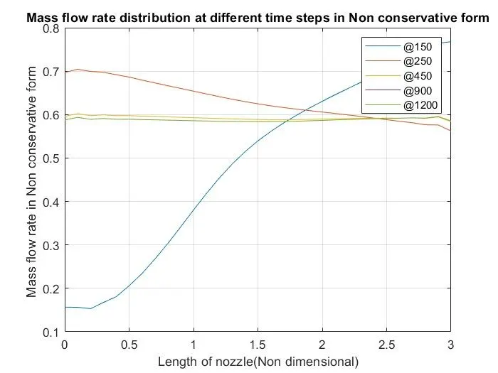
• Variation of mass flow rate distribution inside the nozzle at different time steps during the time marching process in Non-conservative form:

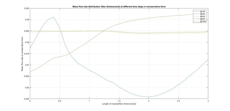
• Variation of Mass flow rate distribution inside the nozzle at different time steps during the time marching process in Conservative form:

• Steady -state distribution of primitive variable inside the nozzle at throat in Non - conservative form:

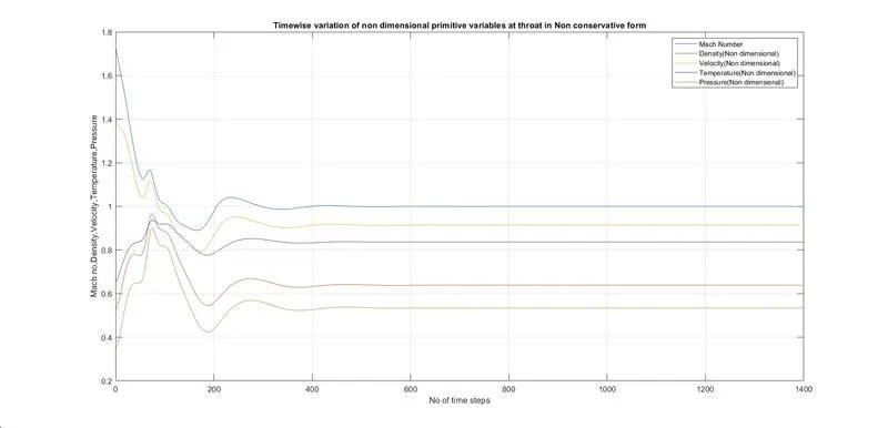
• Steady -state distribution of primitive variable inside the nozzle at throat in Conservative form:

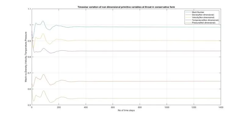
• Steady -state distribution of primitive variable inside the nozzle in Non - conservative form:

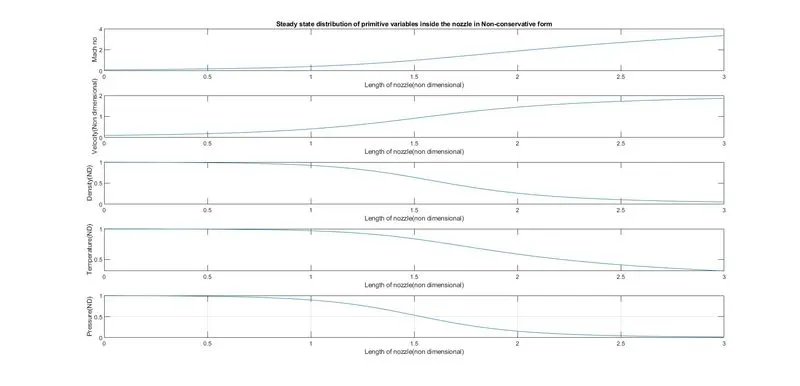
• Steady -state distribution of primitive variable inside the nozzle in Conservative form:

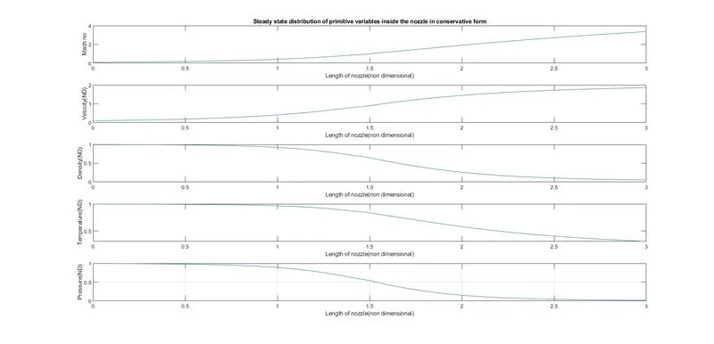
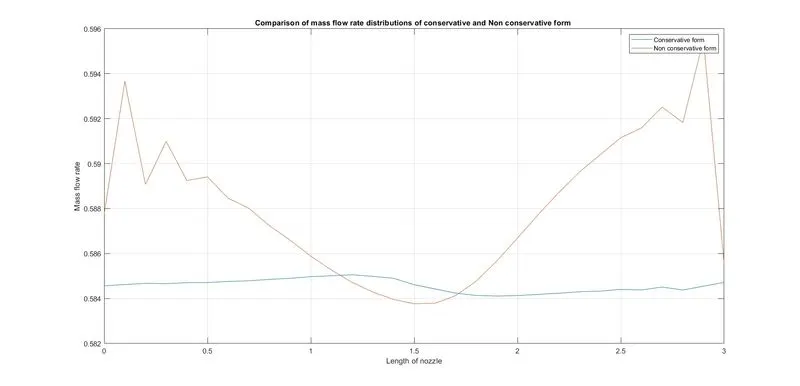
• Comparison of Normlized mass flow rate distributions of Non conservative and conservative forms:

Explanation:

• The above figure shows that the mass flow rate distribution of both non-conservative and conservative form.
• The comparison shown in above plot is illustrate the general advantage of Conservative form of the equations.
• The conservative form does a better job of preserving mass throughout the flow field,mainly because the mass flow itself is one of the dependent variables in the equations,the mass flow is a primary result from these equations .In contrast ,the dependent variables and the mass flow is obtained only as a secondary result.because the conservative form of the equations does a better job of conserving mass throughout the flow field,we can begin to understand why they are labeled the conservative form

Simulation Time:

Execution time for Non Conservative form(Time_Nc)=1.7259 sec

Execution time for Conservative form(Time_c)=1.8785 sec

Grid Independence Test:

For Number of grid points (n)=31

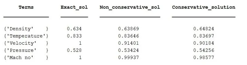
• The obtained solutions results are approximately matching with the exact solution,hence the grid can be considered as grid independent
• The above figure shows the grid indepependence test results,We observed that the Non conservative form give more accurate result than the conservative form.If we doubled the grid points and result checked then the steady state numerical results are slightly closer to the exact,analytical values but still not as close as the non conservation form results with half as many grid points.For all practical purposes ,we have grid independence with 31 grid points.

Conclusion: