Week 3.5 - Deriving 4th order approximation of a 2nd order derivative using Taylor Table method

Aim:-

Derive the following 4th order approximations of the second-order derivative.

1. Central difference

2. Skewed right-sided difference

3. Skewed left-sided difference

After deriving these schemes, prove that your skewed schemes are fourth-order accurate

write a program in Matlab to evaluate the second-order derivative of the analytical function exp(x)*cos(x) and compare it with the 3 numerical approximations that you have derived.

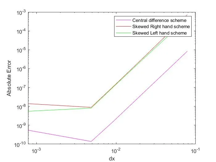
Provide a plot that compares the absolute error between the above-mentioned schemes

In your own words, describe why a skewed scheme is useful? What can a skewed scheme do that a CD scheme cannot?

Procedure:-

Derivation

1) Central Difference scheme

The numerical stencil for central Difference Scheme is

(i-2)-----------(i-1)-----------(i)-----------(i+1)-----------(i+2)

For central difference scheme the double derivative can be written as follows

`(d^2y)/(dx^2)=af(i-2)+bf(i-1)+cf(i)+df(i+1)+ef(i+2)`-----------(1) `

Using Taylor Series we can expand the above equation as follows,

`af(i-2)=a(f(i)-2 Deltaxf'(i)+((2 Deltax)^2f''(i))/(2!)-((2 Deltax)^3f^(iii)(i))/(3!)+((2 Deltax)^4f^(iv)(i))/(4!))`

`bf(i-1)=b(f(i)- Deltaxf'(i)+(( Deltax)^2f''(i))/(2!)-((Deltax)^3f^(iii)(i))/(3!)+(( Deltax)^4f^(iv)(i))/(4!))`

`df(i+1)=d(f(i)+ Deltaxf'(i)+(( Deltax)^2f''(i))/(2!)+((Deltax)^3f^(iii)(i))/(3!)+(( Deltax)^4f^(iv)(i))/(4!))`

`ef(i+2)=e(f(i)+2 Deltaxf'(i)+((2 Deltax)^2f''(i))/(2!)+((2 Deltax)^3f^(iii)(i))/(3!)+((2 Deltax)^4f^(iv)(i))/(4!))`

from the taylor Table the value of the coefficient can be found,

	f(i)	`Deltaxf'(i)`	`Deltax^2f''(i)`	`Deltax^3f^(iii)(i)`	`Deltax^4f^(iv)(i)`
`af(i-2)`	a	-2a	(4/2)*a	-(8/6)*a	(16/24)*a
`bf(i-1)`	b	-b	b/2	-b/6	b/24
`cf(i)`	c	0	0	0	0
`df(i+1)`	d	d	d/2	d/6	d/24
`ef(i+2)``	e	2e	(4/2)*e	(8/6)*e	(16/24)*e
Sum of Coefficient	0	0	1	0	0

from taylor table we have found equation

a+b+c+d+e=0

-2a-b+d+2e=0

2*a+b/2+d/2+2e=1

-(4/3)*a-b/6+d/6+(4/3)*e=0

(2/3)*a+b/24+d/24+(2/3)*e=0

Converting above equation in matrix form

A1=[1 1 1 1 1;-2 -1 0 1 2 ;2 0.5 0 0.5 2;-4/3 -1/6 0 1/6 4/3; 2/3 1/24 0 1/24 2/3]

B1=[0;0;1;0;0]

X1=[a;b;c;d;e]

Consider A1X1=B1

by solving above equation by matrix inversion method in matlab we get,

a= -0.0833

b= 1.3333

c=-2.5000

d=1.3333

e=-0.0833

Hence a=e,b=d

equation (1) becomes

`af(i-2)+bf(i-1)+cf(i)+df(i+1)+ef(i+2)=Deltax^2f''(i)`

`f''(i)=((af(i-2)+bf(i-1)+cf(i)+df(i+1)+ef(i+2)))/(Deltax^2)`

This the expression for central Difference scheme.

2) Skewed Right hand scheme :

The numerical stencil for Skewed Right hand Scheme is

(i)-----------(i+1)-----------(i+2)-----------(i+3)-----------(i+4)-----------(i+5)

For Skewed Right hand scheme the double derivative can be written as follows

`(d^2y)/(dx^2)=af(i)+bf(i+1)+cf(i+2)+df(i+3)+ef(i+4)+gf(i+5)`-----------(2) `

Using Taylor Series we can expand the above equation as follows,

`bf(i+1)=b(f(i)+ Deltaxf'(i)+(( Deltax)^2f''(i))/(2!)+(( Deltax)^3f^(iii)(i))/(3!)+((Deltax)^4f^(iv)(i))/(4!)+((Deltax)^5f^(v)(i))/(5!))`

`cf(i+2)=c(f(i)+2 Deltaxf'(i)+((2 Deltax)^2f''(i))/(2!)+((2Deltax)^3f^(iii)(i))/(3!)+((2 Deltax)^4f^(iv)(i))/(4!)+((2 Deltax)^5f^(v)(i))/(5!))`

`df(i+3)=d(f(i)+3 Deltaxf'(i)+((3 Deltax)^2f''(i))/(2!)+((3Deltax)^3f^(iii)(i))/(3!)+((3 Deltax)^4f^(iv)(i))/(4!)+((3 Deltax)^5f^(v)(i))/(5!))`

`ef(i+4)=e(f(i)+4 Deltaxf'(i)+((4 Deltax)^2f''(i))/(2!)+((4Deltax)^3f^(iii)(i))/(3!)+((4 Deltax)^4f^(iv)(i))/(4!)+((4 Deltax)^5f^(v)(i))/(5!))`

`gf(i+5)=g(f(i)+5 Deltaxf'(i)+((5Deltax)^2f''(i))/(2!)+((5Deltax)^3f^(iii)(i))/(3!)+((5 Deltax)^4f^(iv)(i))/(4!)+((5 Deltax)^5f^(v)(i))/(5!))`

from the taylor Table the value of the coefficient can be found,

	f(i)	`Deltaxf'(i)`	`Deltax^2f''(i)`	`Deltax^3f^(iii)(i)`	`Deltax^4f^(iv)(i)`	`Deltax^5f^(v)(i)`
`af(i)`	a	0	0	0	0	0
`bf(i+1)`	b	b	b/2	b/6	b/24	b/120
`cf(i+2)`	c	2c	2c	(4/3)*c	(16/24)c	(32/120)*c
`df(i+3)`	d	3d	(9/2)*d	(9/2)*d	(81/24)*d	(243/120)*d
`ef(i+4)`	e	4e	8e	(32/3)*e	(256/24)*e	(1024/120)*e
`gf(i+5)``	g	5g	(25/2)*g	(125/6)*g	(625/24)*g	(3125/120)*g
Sum of Coefficient	0	0	1	0	0	0

from taylor table we have found equation

a+b+c+d+e+g=0

b+2c+3d+4e+5g=0

(b/2)+2c+(9/2)*d+8e+(25/2)*g=1

b/6+(4/3)*c+(9/2)*d+(32/3)*e+(125/6)*g=0

b/24+(16/24)*c+(81/24)*d+(256/24)*e+(625/24)*g=0

b/120+(32/120)*c+(243/120)*d+(1024/120)*e+(3125/120)*g=0

Converting above equation in matrix form

A2=[1 1 1 1 1 1;0 1 2 3 4 5 ;0 1/2 2 9/2 8 25/2 ;0 1/6 4/3 9/2 32/3 125/6 ;0 1/24 16/24 81/24 256/24 625/24; 0 1/120 32/120 243/120 1024/120 3125/120]

B2=[0;0;1;0;0;0]

X2=[a;b;c;d;e;g]

Consider A2X2=B2

by solving above equation by matrix inversion method in matlab we get,

a=3.7500

b= -12.8333

c=17.8333

d=-13.0000

e=5.0833

g=-0.8333

We have

`af(i)+bf(i+1)+cf(i+2)+df(i+3)+ef(i+4)+gf(i+5)=Deltax^2f''(i)`

`f''(i)=(af(i)+bf(i+1)+cf(i+2)+df(i+3)+ef(i+4)+gf(i+5))/(Deltax^2)`

This is the expression for Skewed right hand scheme.

3) Skewed Left hand scheme :

The numerical stencil for Skewed left hand Scheme is

(i-5)-----------(i-4)-----------(i-3)-----------(i-2)-----------(i-1)-----------(i)

For Skewed left hand scheme the double derivative can be written as follows

`(d^2y)/(dx^2)=af(i-5)+bf(i-4)+cf(i-3)+df(i-2)+ef(i-1)+gf(i)`-----------(3) `

Using Taylor Series we can expand the above equation as follows,

`af(i-5)=a(f(i)- 5Deltaxf'(i)+(( 5Deltax)^2f''(i))/(2!)-(( 5Deltax)^3f^(iii)(i))/(3!)+((5Deltax)^4f^(iv)(i))/(4!)-((5Deltax)^5f^(v)(i))/(5!))`

`bf(i-4)=b(f(i)- 4Deltaxf'(i)+(( 4Deltax)^2f''(i))/(2!)-(( 4Deltax)^3f^(iii)(i))/(3!)+((4Deltax)^4f^(iv)(i))/(4!)-((4Deltax)^5f^(v)(i))/(5!))`

`cf(i-3)=c(f(i)- 3Deltaxf'(i)+(( 3Deltax)^2f''(i))/(2!)-(( 3Deltax)^3f^(iii)(i))/(3!)+((3Deltax)^4f^(iv)(i))/(4!)-((3Deltax)^5f^(v)(i))/(5!))`

`df(i-2)=d(f(i)- 2Deltaxf'(i)+(( 2Deltax)^2f''(i))/(2!)-(( 2Deltax)^3f^(iii)(i))/(3!)+((2Deltax)^4f^(iv)(i))/(4!)-((2Deltax)^5f^(v)(i))/(5!))`

`ef(i-1)=e(f(i)- Deltaxf'(i)+(( Deltax)^2f''(i))/(2!)-(( Deltax)^3f^(iii)(i))/(3!)+((Deltax)^4f^(iv)(i))/(4!)-((Deltax)^5f^(v)(i))/(5!))`

from the taylor Table the value of the coefficient can be found,

	f(i)	`Deltaxf'(i)`	`Deltax^2f''(i)`	`Deltax^3f^(iii)(i)`	`Deltax^4f^(iv)(i)`	`Deltax^5f^(v)(i)`
`af(i-5)`	a	-5a	(25/2)*a	(-125/6)*a	(625/24)*a	(-3125/120)*a
`bf(i-4)`	b	-4b	(16/2)*b	(-64/6)*b	(256/24)*b	(-1024/120)*b
`cf(i-3)`	c	-3c	(9/2)*c	(-27/6)*c	(81/24)*c	(-243/120)*c
`df(i-2)`	d	-2d	(4/2)*d	(-8/6)*d	(16/24)*d	(-32/120)*d
`ef(i-1)`	e	-e	(e/2)	(-e/6)	(e/24)	(-e/120)
`gf(i)`	g	0	0	0	0	0
Sum of Coefficient	0	0	1	0	0	0

from taylor table we have found equation

a+b+c+d+e+g=0

-5a-4b-3c-2d-e=0

(25/2)*a+(16/2)*b+(9/2)*c+(4/2)*d+(e/2)=1

(-125/6)*a+(-64/6)*b+(-27/6)*c+(-8/6)*d+(-e/6)=0

(625/24)*a+(256/24)*b+(81/24)*c+(16/24)*d+(e/24)=0

(-3125/120)*a+(-1204/120)*b+(-243/120)*c+(-32/120)*d+(-e/120)=0

A3=[1 1 1 1 1 1;-5 -4 -3 -2 -1 0 ;25/4 16/2 9/2 4/2 1/2 0;-125/6 -64/6 -27/6 -8/6 -1/6 0 ;625/24 256/24 81/24 16/24 1/24 0;-3125/120 -1024/120 -243/120 -32/120 -1/120 0]

B3=[0;0;1;0;0;0]

X3=[a;b;c;d;e;g]

Consider A3X3=B3

by solving above equation by matrix inversion method in matlab we get,

a=-0.8333

b= 5.0833

c=-13.0000

d=17.8333

e=-12.8333

g=3.7500

we have

`af(i-5)+bf(i-4)+cf(i-3)+df(i-2)+ef(i-1)+gf(i)=Deltax^2f''(i)`

`f''(i)=(af(i-5)+bf(i-4)+cf(i-3)+df(i-2)+ef(i-1)+gf(i))/(Deltax^2)`

This is the expression for Skewed Left hand scheme.

Matlab Code

clear all
close all
clc
% Analytical function = exp(x)*cos(x)
x=pi/3;
% Analytical Second Derivative of function is
Analytical_Second_Derivative=(-2)*exp(x)*sin(x);
% calculating coefficient of the central difference scheme
%A1=[1 1 1 1 1;-2 -1 0 1 2 ;2 1/2 0 1/2 2;-4/3 -1/6 0 1/6 4/3; 2/3 1/24 0 1/24 2/3];
A1=[1 1 1 1 1;-2 -1 0 1 2 ;2 1/2 0 1/2 2;-4/3 -1/6 0 1/6 4/3; 2/3 1/24 0 1/24 2/3];
B1=[0;0;1;0;0];
X1=linsolve(A1,B1);
% calculating coefficient of the Skewed Right hand scheme
%A2=[1 1 1 1 1 1;0 1 2 3 4 5 ;0 1/2 2 9/2 8 25/2 ;0 1/6 4/3 9/2 32/3 125/6 ;0 1/24 16/24 84/24 256/24 625/24; 0 1/120 32/120 243/120 1024/120 3125/120];
A2=[1 1 1 1 1 1;0 1 2 3 4 5;0 1/2 4/2 9/2 16/2 25/2;0 1/6 8/6 27/6 64/6 125/6;0 1/24 16/24 81/24 256/24 625/24;0 1/120 32/120 243/120 1024/120 3125/120;];
B2=[0;0;1;0;0;0];
X2=linsolve(A2,B2);
% calculating coefficient of the Skewed Left hand scheme
%A3=[1 1 1 1 1 1;-5 -4 -3 -2 -1 0 ;25/4 16/2 9/2 4/2 1/2 0;-125/6 -64/6 -27/6 -8/6 -1/6 0 ;625/24 256/24 81/24 16/24 1/24 0;-3125/120 -1204/120 -243/120 -32/120 -1/120 0];
A3=[1 1 1 1 1 1;-5 -4 -3 -2 -1 0;25/2 16/2 9/2 4/2 1/2 0;-125/6 -64/6 -27/6 -8/6 -1/6 0;625/24 256/24 81/24 16/24 1/24 0;-3125/120 -1024/120 -243/120 -32/120 -1/120  0];
B3=[0;0;1;0;0;0];
X3=linsolve(A3,B3);
% Numerical Derivatives for the given schemes are 
dx=linspace(pi/40,pi/4000,20);
for i=1:length(dx)
 %CDS(i)=((X1(1)*exp(x-(2*dx(i)))*cos(x-(2*dx(i)))))+(X1(2)*exp(x-(dx(i)))*cos(x-(dx(i))))+(X1(3)*exp(x)*cos(x))+(X1(4)*exp(x+(dx(i)))*cos(x+(dx(i))))+(X1(5)*exp(x+(2*dx(i)))*cos(x+(2*dx(i))))/(dx(i)^2);
 CDS(i)=(((X1(1)*exp(x-(2*dx(i)))*cos(x-(2*dx(i)))))+(X1(2)*exp(x-(dx(i)))*cos(x-(dx(i))))+(X1(3)*exp(x)*cos(x))+(X1(4)*exp(x+(dx(i)))*cos(x+(dx(i))))+(X1(5)*exp(x+(2*dx(i)))*cos(x+(2*dx(i)))))/(dx(i)^2);
 %Skewed_right(i)=(X2(1)*exp(x)*cos(x))+(X2(2)*exp(x+(dx(i)))*cos(x+(dx(i))))+((X2(3)*exp(x+(2*dx(i)))*cos(x+(2*dx(i)))))+(X2(4)*exp(x+(3*dx(i)))*cos(x+(3*dx(i))))+((X2(5)*exp(x+(4*dx(i)))*cos(x+(4*dx(i)))))+((X2(6)*exp(x+(5*dx(i)))*cos(x+(5*dx(i)))))/(dx(i)^2);
 Skewed_right(i)=((X2(1)*exp(x)*cos(x))+(X2(2)*exp(x+(dx(i)))*cos(x+(dx(i))))+((X2(3)*exp(x+(2*dx(i)))*cos(x+(2*dx(i)))))+(X2(4)*exp(x+(3*dx(i)))*cos(x+(3*dx(i))))+((X2(5)*exp(x+(4*dx(i)))*cos(x+(4*dx(i)))))+((X2(6)*exp(x+(5*dx(i)))*cos(x+(5*dx(i))))))/(dx(i)^2);
 %Skewed_left(i)=((X3(1)*exp(x-(5*dx(i)))*cos(x-(5*dx(i)))))+((X3(2)*exp(x-(4*dx(i)))*cos(x-(4*dx(i)))))+((X3(3)*exp(x-(3*dx(i)))*cos(x-(3*dx(i)))))+((X3(4)*exp(x-(2*dx(i)))*cos(x-(2*dx(i)))))+((X3(5)*exp(x-(dx(i)))*cos(x-(dx(i)))))+(X3(6)*exp(x)*cos(x))/(dx(i)^2);
 Skewed_left(i)=(((X3(1)*exp(x-(5*dx(i)))*cos(x-(5*dx(i)))))+((X3(2)*exp(x-(4*dx(i)))*cos(x-(4*dx(i)))))+((X3(3)*exp(x-(3*dx(i)))*cos(x-(3*dx(i)))))+((X3(4)*exp(x-(2*dx(i)))*cos(x-(2*dx(i)))))+((X3(5)*exp(x-(dx(i)))*cos(x-(dx(i)))))+(X3(6)*exp(x)*cos(x)))/(dx(i)^2);
 % To calculate Absolute Error
 Error_CDS(i)=abs(CDS(i)-Analytical_Second_Derivative);
 Error_Skewed_right(i)=abs(Skewed_right(i)-Analytical_Second_Derivative);
 Error_Skewed_left(i)=abs(Skewed_left(i)-Analytical_Second_Derivative);
end
loglog(dx,Error_CDS,'m')
hold on
loglog(dx,Error_Skewed_right,'r')
hold on
loglog(dx,Error_Skewed_left,'g')
legend('Central difference scheme','Skewed Right hand scheme','Skewed Left hand scheme' )
xlabel('dx')
ylabel('Absolute Error')

The explanation of above matlab code is as follows

Step 1) Take given analytical function and given x value to calculate the analytical second derivative .

Step 2) Take analytical second order derivative of given analytical function

Step 3) To calculate the coefficient of the central Difference scheme, from taylor table we got 5 equations ,this equation is solved by matrix inversion method or in matlab by using linsolve ie inbuilt function to solve the linear equation .

Step 4) by using the procedure of step 3 we calculate the coefficient of skewed right hand and skewed left hand scheme with the help of taylor table .

Step 5) To calculate the numerical derivative of the given three schemes,Assume the dx value we assume the dx value by using linspace command start point is pi/40 and end point is pi/4000 and and make 20 equally spaced element for that dx value.

Step 6) By using For loop calculate the numerical derivative for the Central Difference Scheme,Skewed Right hand Scheme,Skewed Left hand scheme

Step 7) To calculate the absolute error for the Central Difference Scheme,Skewed Right hand Scheme,Skewed Left hand scheme by using the formula which is mentioned in above matlab code .

Step 8) By using loglog plot we plot the graph of Central Difference Scheme,Skewed Right hand Scheme,Skewed Left hand scheme which shows the relation between them for absolute error.

Result:

The graph of Central Difference Scheme,Skewed Right hand Scheme,Skewed Left hand scheme which shows the relation between them for absolute error.

Conclusion:

• The above graph shows that for the value of dx the central difference scheme gives the very less error as compared to the Skewed right and skewed left hand difference scheme.CDS utilizes the available information from left and right ie both the sides.CDS gives the higher order of approximation hence order of approximation increases the absolute error decreases.
• The error decreasing rate for Skewed right and Central Difference scheme is same but for skewed left hand scheme it is comparatively low
• In skewed scheme the information used is from right and left side from successive neighbouring points there error occure is higher than all other scheme.Skewed scheme is used to compute higher order approximation.

why a skewed scheme is useful? What can a skewed scheme do that a CD scheme cannot?

• For skewed scheme in order to obtain the result the information required is collected from left or right side of a given reference point.
• If we requird the result of a boundary side in that incident we cannot have much information from both the sides the information is available at that time is only from one side at that time we use Skewed left or right scheme(depending upon the information) to obtain the desired result.
• Centre difference scheme required information from both the side from a given reference point so to get result for a boundary side CD scheme cannot be used for that.
• At last we concluded that the CD scheme gives the less error but skewed scheme has their own significance when time comes to compute the things at boundary or insufficient availability of information.