Week 6 - CHT Analysis on a Graphics card

CHT Analysis on a Graphics card

Problem statement:

Perform a steady-state conjugate heat transfer analysis on a model of a graphics card. You can use appropriate materials of your choice for the simulation. Make sure to properly define the correct solid and fluid zones. Refer the video for further clarification and the model is provided below the video.

Run the simulation for best possible mesh with combination of coarse and refined mesh in different regions. Explain the reason for choosing the particular mesh settings.

Objectives:

1. Run the simulation by varying the velocity from 1m/sec to 5m/sec for at least 3 velocities and discuss the results.
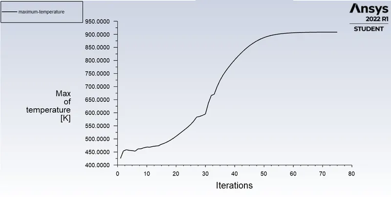
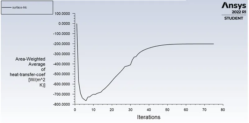
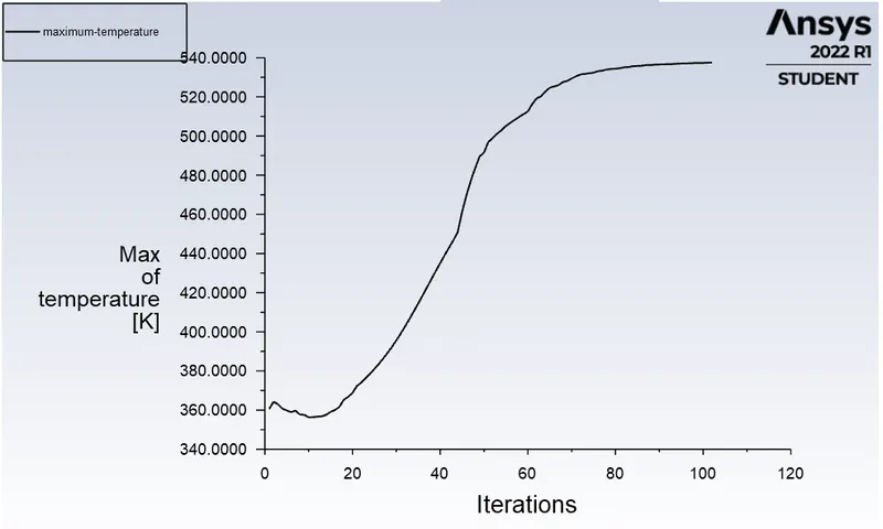
2. Find out the maximum temperature and heat transfer coefficient attained by the processor.
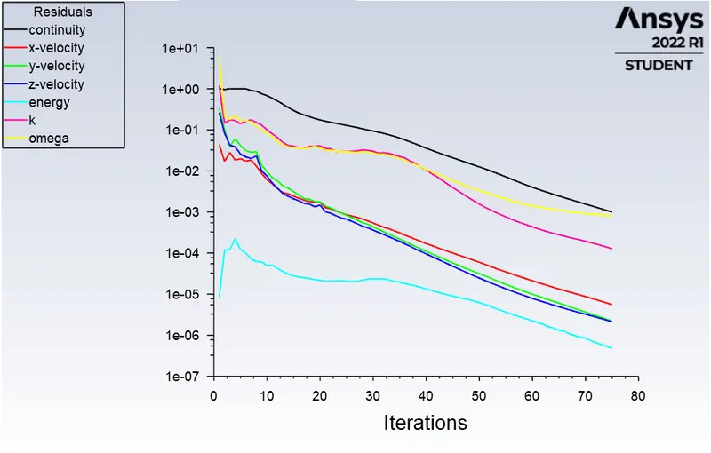
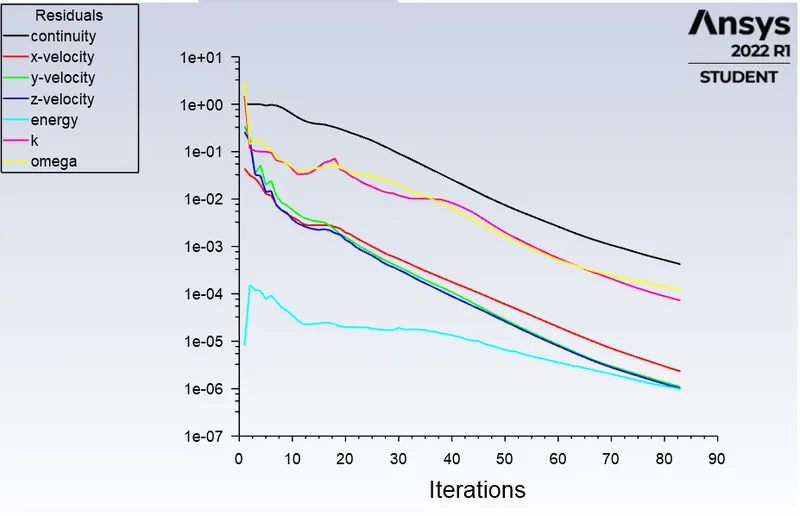
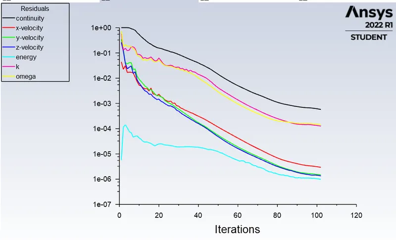
3. Prove that the simulation has achieved convergence with appropriate images and plots.
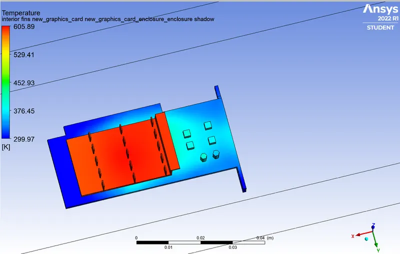
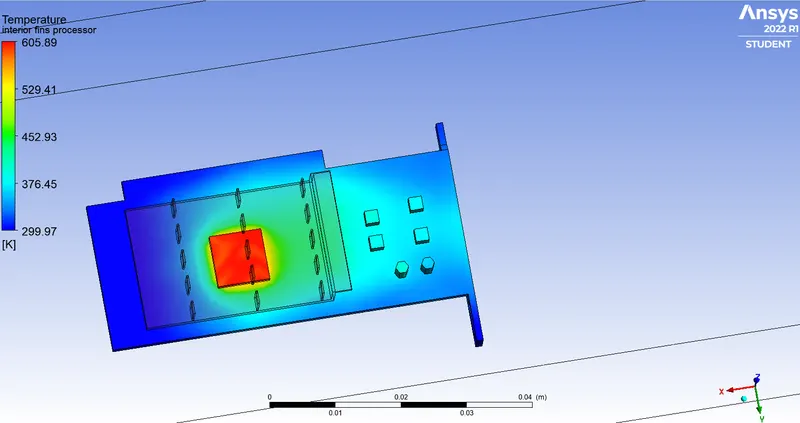
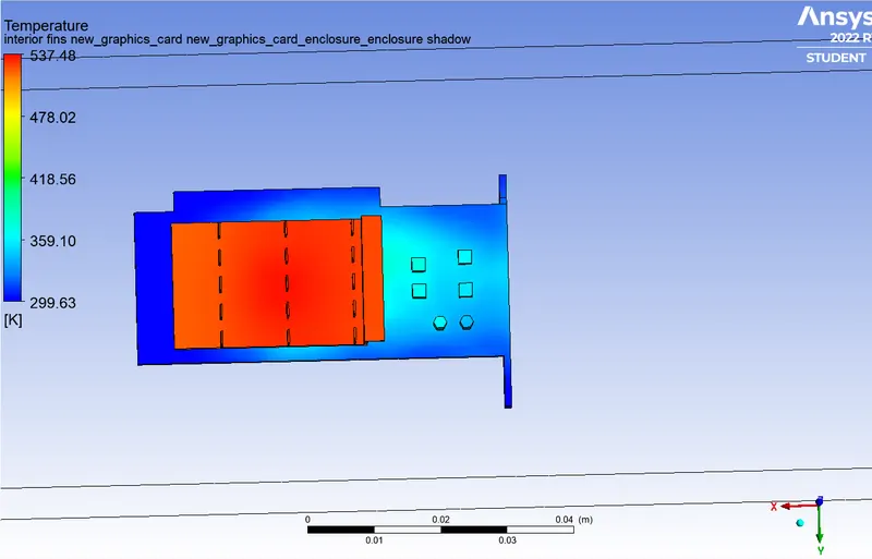
4. Identify potential hotspots on the model.

Procedure:

Theory:

Conjugate Heat transfer:

The conjugate heat transfer analysis type allows for the simulation of heat transfer between solid and fluid domains by exchanging thermal energy at the interfaces between them.Typical applications of this analysis type exit as ,but are not limited to,the simulation of heat exchanger,cooling of electronic equipment,general purpose cooling and heating systems.

Examples:

Internal combustion engine,Heat exchanger,Heat sink,Boiler,Turbocharger etc

Graphics card: The graphics card (video card,display card,display adapter) is a expansion card that generates a feed of output images to a display device (such as a computer monitor ). The integrated graphics processor can perform additional processing ,removing this task from the central processor of the computer.

Step 1) Geometry :

1. The given Graphics card model is open in Spaceclaim. which is in the enclosure.
2. Share topology has to be enabled between the different components so that conformal mesh can be achieved between different components and necessary information can be shared between different zones of the mesh.

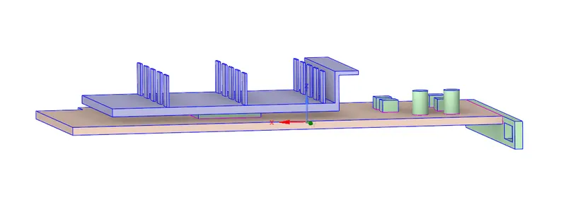
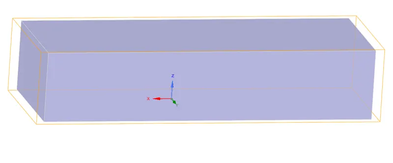
Enclosure:

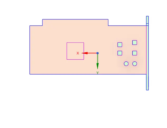
Base:

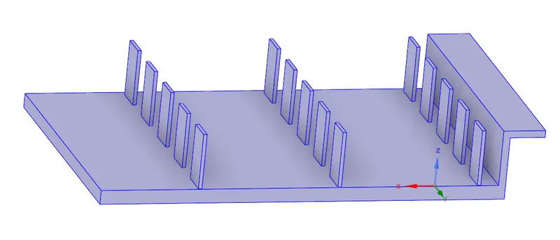
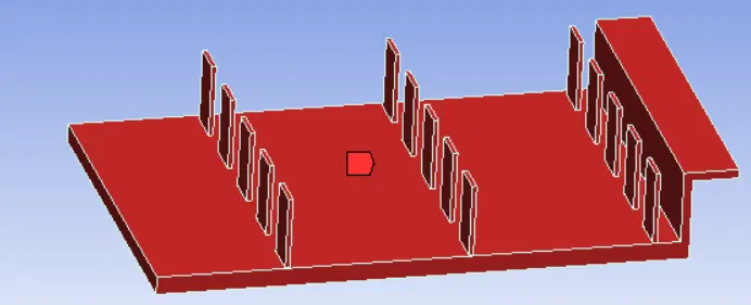
Fins:

Processor:

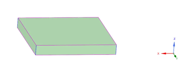
Step 2) Mesh:

Give a name to different parts by using body selection tool :

Fins:

Processor:

Base:

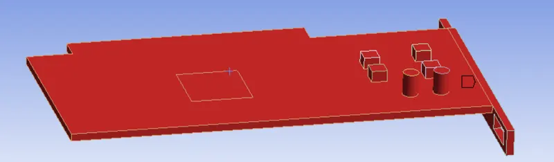
By using face selection tool give a name For enclosure inlet, outlet and for side wall give a name Symmetry wall .

Processor side wall:

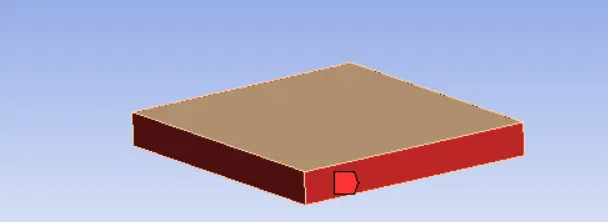
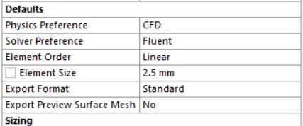
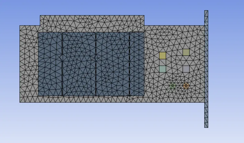
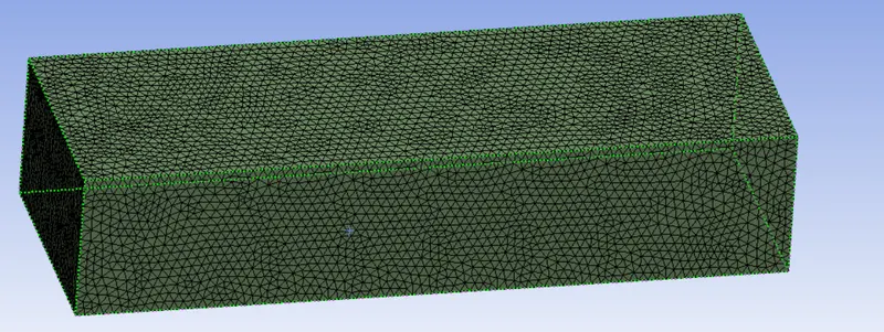
We use element size 2.5mm because the default mesh size is 10.289mm which gives low elemental quality .

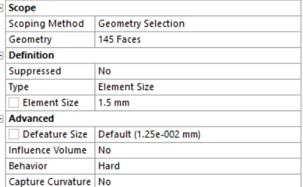
Use face sizing and by using box select tool we select the entire graphics card due to that all the faces are selected and we use element size 1.5 mm

Enclosure:2.5mm

Fins:1.5mm

Base: 1.5mm

Processor: 1.5mm

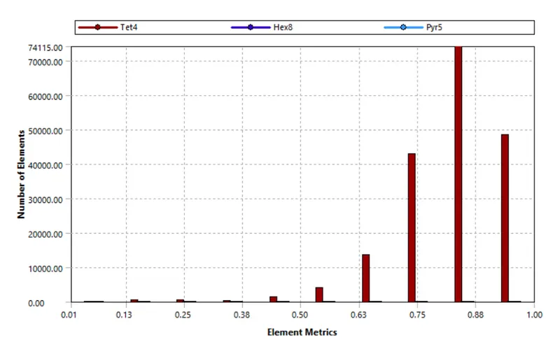
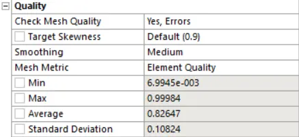
Elemental Quality:

Mesh :

Step 3) Setup and Solution:

• Solver: Steady
• Type: Pressure Based
• Turbulance Model: k-Omega(SST)
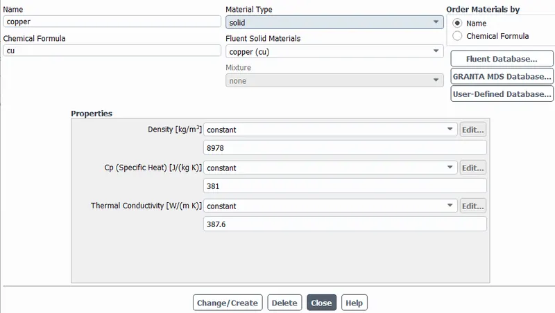
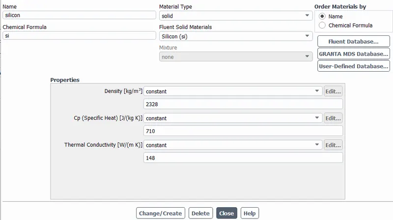
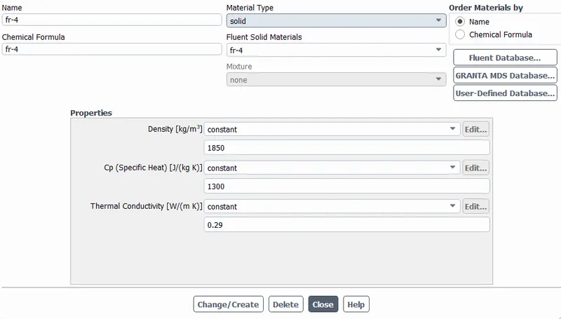
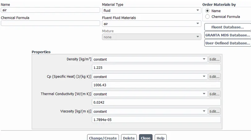
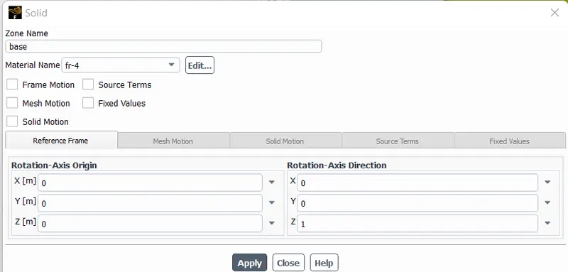
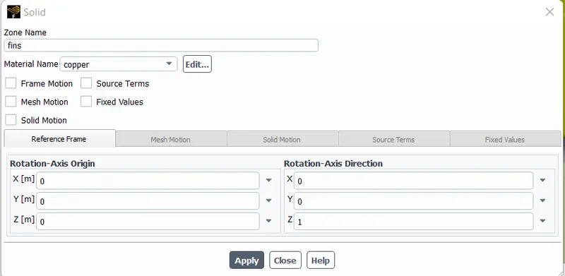
• Materials : Different materials are used for each parts, Some of which are custom created

Parts Material

Fins - Copper

Processor - Silicon (created)

Base - FR-4 (created)

Enclosure - Air

(1) Copper:

(2)Silicon:

(3) FR-4

(4)Air :

Cell zones:

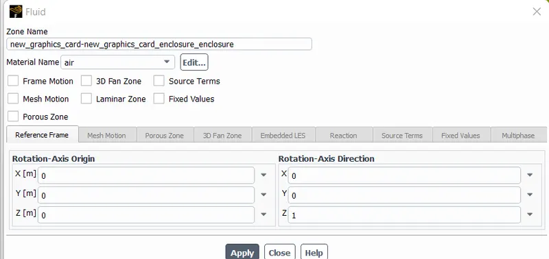
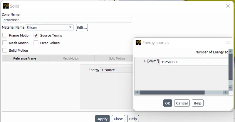
The processor is the only source of heat energy in this case so, The heat energy generated is calculated as ,

Let consider Processor consume 20 W power for work

Volume of the processor :8x8x1= 64`mm^3`=`64*10^-9m^3`

Heat generated : `P/V`=`20`/`64*10^-9`

:312500000 `W/m^3`

Boundaries :

• Inlet:

Type:Velocity inlet

Velocity: 1 m/sec

Temperature:300K

• outlet:

Type:Pressure outlet

Pressure: 0 Pa (gauge pressure)

• symmetry wall

Type: symmetry

• Processor side wall

Type: wall

Method of initialization : Hybrid

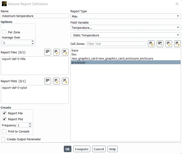
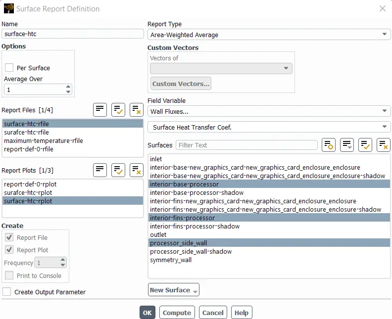
We have to create a report for calculating the maximum temperature,heat transfer coefficient attained by processor.

For maximum Temperature :

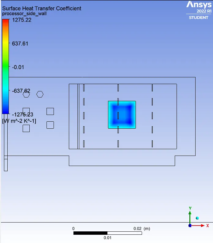
For surface heat transfer coefficient :

Step 4) Result:

Residual plot:

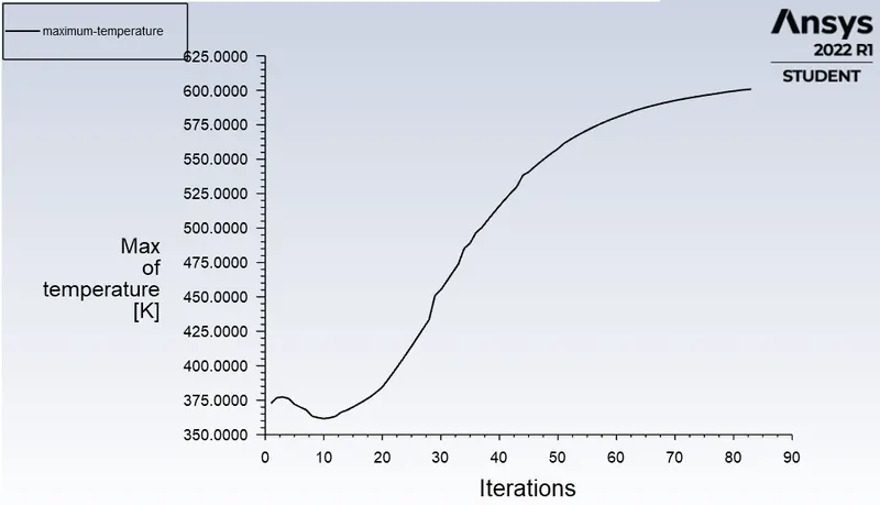
Maximum Temperature plot:

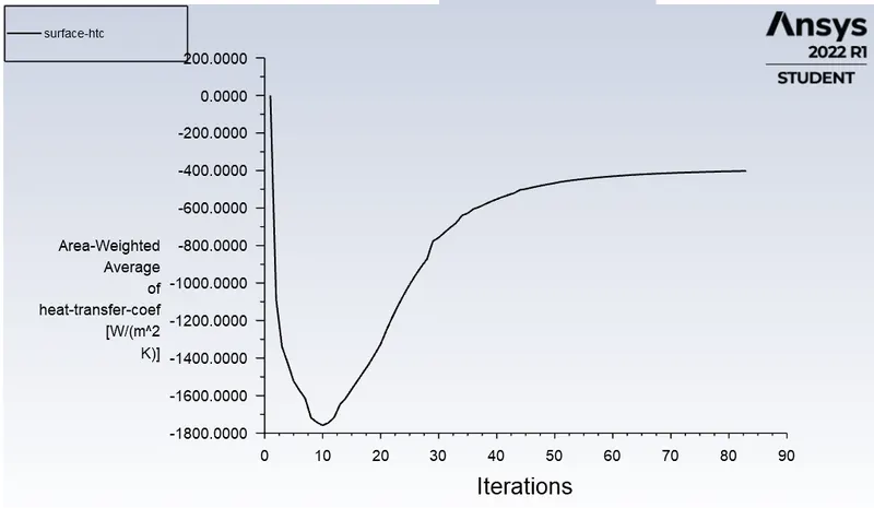
Surface heat transfer Coefficient plot:

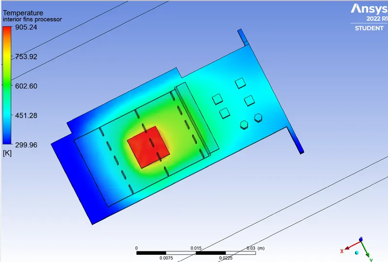
Global Hotspot Region:

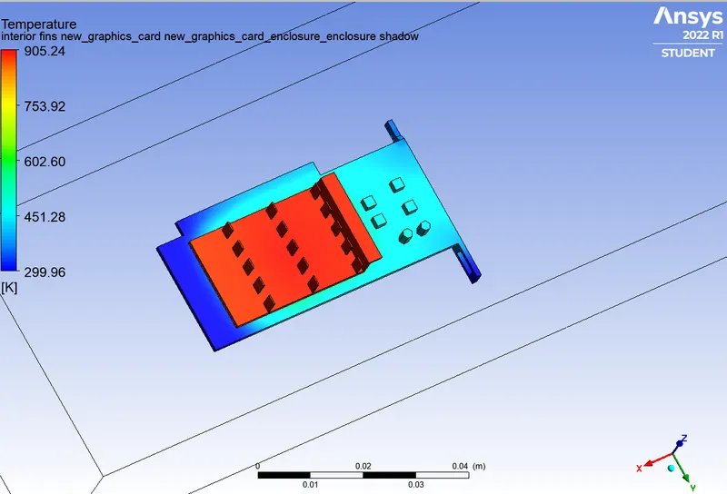
Hotspot around the processor

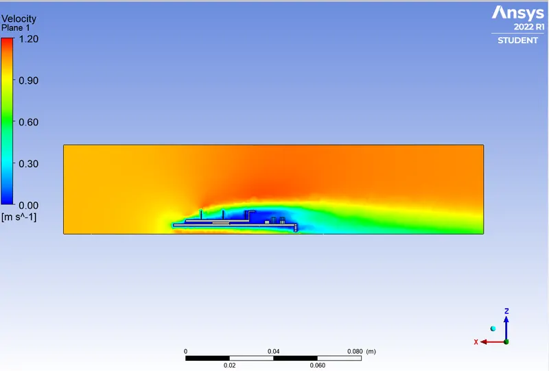
Velocity Contour:

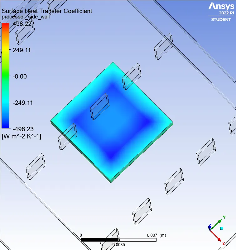
Surface Heat transfer coefficient :

We run the simulation for Velocity 3 m/sec all the set up is same only velocity changed.

Results:

Residual plot:

Maximum Temperature plot:

Surface heat transfer Coefficient plot:

Global Hotspot Region:

Hotspot around the processor:

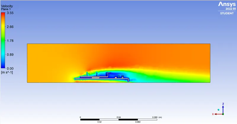
Velocity Contour:

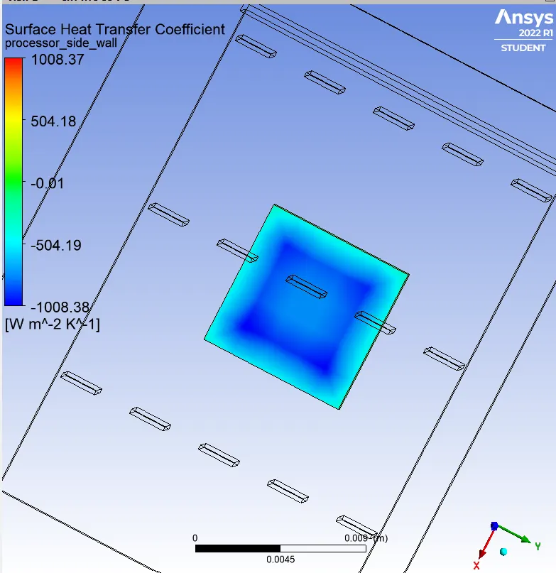
Surface Heat transfer coefficient plot :

For velocity 5 m/sec :

Residual plot:

Maximum Temperature plot:

Surface heat transfer Coefficient plot:

Global Hotspot Region:

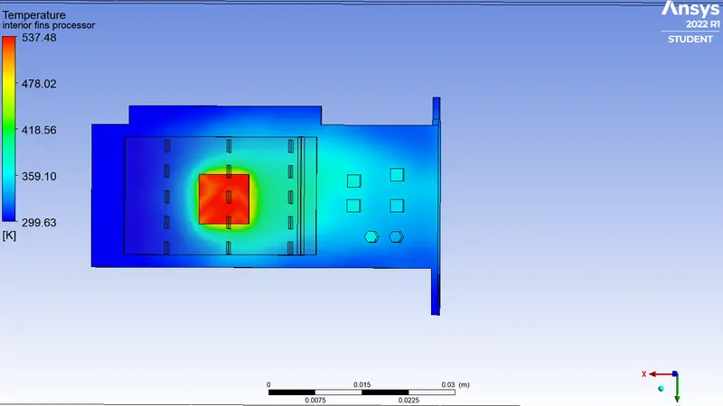
Hotspot around the processor:

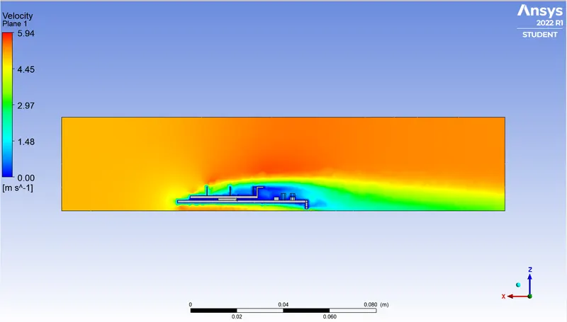
Velocity Contour:

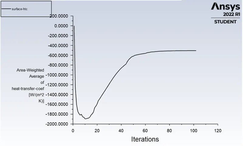
Surface Heat transfer coefficient plot :

Results:

Sr No	Velocity (m/sec)	Maximum Temperature at processor (K)	HTC at processor `(W/(m^2K))`
1	1	908.0522	202.4223
2	3	600.8156	402.6768
3	5	537.5621	505.6494

Conclusion:

1. From the above table we observed that the maximum temperature of the processor is decreasing with an increasing the inlet velocity of air .
2. The surface heat transfer coefficient at processor is increasing as we increase the velocity of air.
3. Hence from that observations we can say that the higher inlet velocity result in better cooling and lower the average temperature thus we can maintain the optimum temperature at processor to avoid the damage of components.