Week 4.1 - Genetic Algorithm

Aim: To write a code in MATLAB to optimise the stalagmite function and find the global maxima of the function.

Objective:

• Explain the concept of genetic algorithm.
• Explain the syntax of ga used in Matlab.
• Plot graphs for all 3 studies and for F maximum vs no. of iterations.

Equation:

`f(x,y)=f_(1x),f_(2x),f_(1y),f_(2y)`

`f_(1x)=[sin(5.1pix+0.5)]^6`

`f_(1y)=[sin(5.1piy+0.5)]^6`

`f_(2x)=exp[-4ln(2)*((x-0.0667)^2)/0.64]`

`f_(2y)=exp[-4ln(2)*((y-0.0667)^2)/0.64]`

Procedure:

Genetic Algorithm:

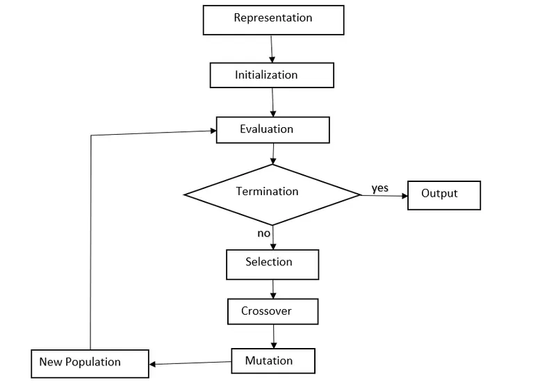
Genetic algorithm is a method for solving both constrained and unconstrained optimization problems that are based on natural selection,the process that drives biological evolution.In computer science and operations researchs, a genetic Algorithm is a metaheauristic inspired by the process of natural selection that belongs to the larger class of evolutionary algorithms(EA). Genetic algorithms are commonly used to generate high-quality solutions to optimization and search problem by relying on biologically inspired operators such as mutation,crossover and selection.

The genetic algorithm is start with the randomly generated population of size M.During the process of iteration ,a new population of a same size is generated from the current population using three basic operations on the individuals of the population .

Five phases are considered in a genetic algorithm

1) Initial population

2) Fitness function

3) Selection

4) Crossover

5) mutation

1) Initial population:

• The process begin with a set of individual which is called population.Each individual is solution to the problem you want to solve.
• An individual is characterized by set of parameter (variables) known as genes.Genes are joined by string to form a chromosome (solution).

2) Fitness Function:

• The Fitness Function determines how fit an individual is. It gives a fitness score to each individual .The probability that an individual will be selected for reproduction is based on its score .

3) Selection:

• The idea of the selection phase is to select the fittest individual and let them pass their genes to the next generation.
• Two pairs of individual are selected based on their fitness score.

4) Crossover:

• Crossover is most significant phase in a genetic algorithm.For a each pair of parents to be mated, a cross over point is chosen at random from within the genes.

5) Mutation :

• In a certain new offspring formed, some of their genes can be subjected to a mutation with low random probability .This implies that some of the bits in the bit string can be flipped.

Syntax of GA

x= ga(fun,nvars)

x=ga(fun,nvars,A,b)

x=ga(fun,nvars,A,b,Aeq,beq)

x=ga(fun,nvars,A,b,Aeq,beq,lb,ub)

x=ga(fun,nvars,A,b,Aeq,beq,lb,ub,nonlcon)

x=ga(fun,nvars,A,b,Aeq,beq,lb,ub,nonlcon,options)

x=ga(fun,nvars,A,b,Aeq,beq,lb,ub,nonlcon,intcon)

x=ga(fun,nvars,A,b,Aeq,beq,lb,ub,nonlcon,intcon,options)

x=ga(problem)

[x,fval]=ga(--)

here,

Inputs Arguments:

fun= Objective function

nvars=Number of variables

A=Linear inequality constraints

b= Linear inequality constraints

Aeq=Linear equality constraints

beq=Linear equality constraints

lb=Lower bound

ub=Upper bound

nonlcon=Non linear constraints

options=Integer variables

problem=Problem descriptions

Output Argument

x=solution

fval=Objective function value at the solution

Matlab code for evaluating the stalagmite function:

clear all
close all
clc
%Defining our search path 
x=linspace(0,0.6,150);
y=linspace(0,0.6,150);
% Creating the 2D mesh
[xx yy]=meshgrid(x,y);
% Evaluating the stalagmite function 
for i=1:length(xx)
        for j=1:length(yy)
            input_vector(1)=xx(i,j);
            input_vector(2)=yy(i,j);
            f(i,j)=stalagmite(input_vector);
        end
end
%For visualize the surface plot
surfc(xx,yy,-f)
xlabel('x values')
ylabel('y values')
shading interp
[input,fval]=ga(@stalagmite,2)

Explanation of above code is follows:

Step 1) Defining our search path, define the x and y array with the help of linspace command.

Step 2) Creating the 2 Dimensional mesh using meshgrid command

Step 3)Evaluating the stalagmite function,we use for loop

Step 4) We use surfc command for visualize the surface plot

Function Code

function [f]=stalagmite(input_vector)
x=input_vector(1);
y=input_vector(2);

f1=(sin(5.1*pi*x+0.5))^6;
f2=(sin(5.1*pi*y+0.5))^6;
f3=exp(-4*log(2)*(x-0.0667)^2/0.64);
f4=exp(-4*log(2)*(y-0.0667)^2/0.64);

f=-(f1*f2*f3*f4);
end

we use - ve sign in above code due to the finding of maximum value .

output:

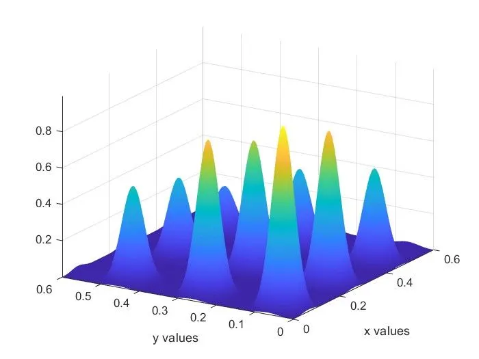
Matlab code for 3 study we have done for finding the global maxima:

clear all
close all
clc

x=linspace(0,0.6,150);
y=linspace(0,0.6,150);
[xx,yy]=meshgrid(x,y);
num_cases =50
for i=1:length(xx)
        for j=1:length(yy)
            input_vector(1)=xx(i,j);
            input_vector(2)=yy(i,j);
            f(i,j)=stalagmite(input_vector);
        end
end

% study 1 statistical behaviour 
tic
for i=1:num_cases
    [inputs,fopt(i)]=ga(@stalagmite,2);
    xopt(i)=inputs(1);
    yopt(i)=inputs(2);
end
study1_time=toc
fopt=-fopt;
figure(1)
subplot(2,1,1)
hold on
surfc(xx,yy,-f)
shading interp
plot3(xopt,yopt,fopt,'marker','o','markersize',5,'markerfacecolor','r')
title('Unbounded inputs')
subplot(2,1,2)
plot(fopt)
xlabel('Iterations')
ylabel('function maximum')
tic
% Study 2 Statistical behaviour with upper and lower bounds


for i=1:num_cases
    [inputs,fopt(i)]=ga(@stalagmite,2,[],[],[],[],[0,0],[1,1]);
    xopt(i)=inputs(1);
    yopt(i)=inputs(2);
end
study2_time=toc
fopt=-fopt;
figure(2)
subplot(2,1,1)
hold on
surfc(xx,yy,-f)
shading interp
plot3(xopt,yopt,fopt,'marker','o','markersize',5,'markerfacecolor','r')
title('Bounded inputs')
subplot(2,1,2)
plot(fopt)
xlabel('Iterations')
ylabel('function maximum')

% Study 3- Increasing GA Iterations
options=optimoptions('ga')
options=optimoptions(options,'PopulationSize',500);
tic
for i=1:num_cases
    [inputs,fopt(i)]=ga(@stalagmite,2,[],[],[],[],[0,0],[1,1],[],[],options);
    xopt(i)=inputs(1);
    yopt(i)=inputs(2);
end
study3_time=toc
fopt=-fopt;
figure(3)
subplot(2,1,1)
hold on
surfc(xx,yy,-f)
shading interp
plot3(xopt,yopt,fopt,'marker','o','markersize',5,'markerfacecolor','r')
title('Bounded inputs with increasing ga iterations')
subplot(2,1,2)
plot(fopt)
xlabel('Iterations')
ylabel('function maximum')

Explanation of above code is follows:

Step 1) For Study (1) statistical behaviour, In this case for loop is used to 50 iterations ,During execution of for loop stalagmite function is called with 'ga',respective plot is done,tic and toc command is used to measure the time taken for execution of all the iterations.

Step 2) for Study (2) Statistical behaviour with upper and lower bounds, In this case for loop is used to 50 iterations ,During execution of for loop stalagmite function is called with 'ga',respective plot is done,tic and toc command is used to measure the time taken for execution of all the iterations.

Step 3) For Study (3) Increasing GA Iterations, For loop is executed,During execution of for loop stalagmite function is called with 'ga',Here Optimoption command is used to return ga solver and to define population size ,here tic and toc command is used to measure the time taken for execution of all the iterations.

Results:

1) The plot of Study (1) statistical behaviour

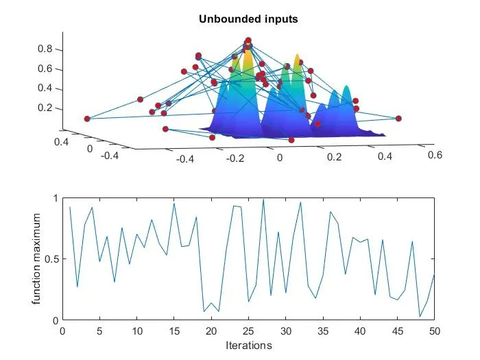
• The above image we shows the two graph in this 1st sub plot we shows the Unbounded inputs
• In 2nd subplot we shows that function maximum values with iteration graph in this 1st study we do not get the maximum value,results is fluctuating.

2) The plot of Study (2) Statistical behaviour with upper and lower bounds,

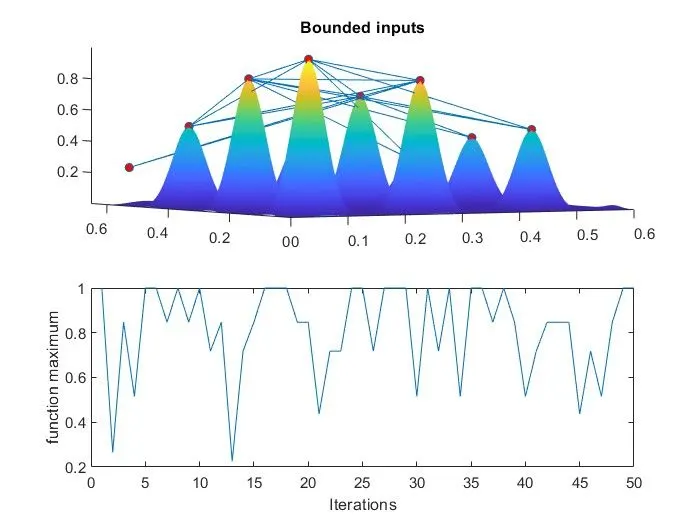
• The above image we shows the two graph in this 1st sub plot we shows the Bounded inputs
• In 2nd subplot we shows that function maximum values with iteration graph in this 2nd study, We get the maximum value for the function for some iteration but the result is also fluctuated in this case also.

3) The plot of Study (3) Increasing GA Iterations,

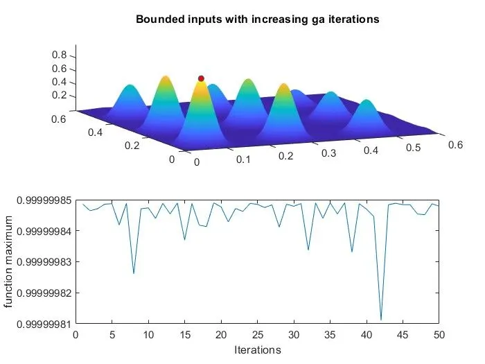
• The above image we shows the two graph in this 1st sub plot we shows the Bounded inputs with increasing the ga Iteration
• In 2nd subplot we shows that function maximum values with iteration graph in this 3rd study, We get the maximum value for the function in range of 0.99999984 to 0.99999985 ie closer to 1 except some iterations
• In this case we use optmoptions command and population size is 500 ,If we increasing population size we also get accurate results even if we run the program for several times.

References:

https://skill-lync.com/knowledgebase/genetic-algorithm-explained

https://in.mathworks.com/help/gads/ga.html

https://en.wikipedia.org/wiki/Stalagmite