Week 5 - Rayleigh Taylor Instability

Objectives:

1. What are some practical CFD models that have been based on the mathematical analysis of Rayleigh Taylor waves? In your own words, explain how these mathematical models have been adapted for CFD calculations.
2. Perform the Rayleigh Taylor instability simulation for 2 different mesh sizes with the base mesh being 0.5 mm. Compare the results by showing the animations( Attach them from your google drive). Observe the differences in the animation and explain the effect of mesh size on simulation. Also, explain why a steady-state approach might not be suitable for these types of simulation.[ Choose Air and Water for this simulation]
3. Run one more simulation with water and user-defined material(density = 400 kg/m³, viscosity = 0.001 kg/m-s) for refined mesh. 
4. Define the Atwood Number. Find out the Atwood number for both the cases and explain how the variation in Atwood number in the above two cases affects the behavior of the instability. 

Procedure:

Introduction:

Rayleigh Taylor Instability :

                                     The Rayleigh–Taylor instability is an instability  of an interface between two fluids of different densities which occurs  when the lighter fluid is pushing the heavier fluid. Examples include the behaviour of water suspended above oil in the gravity of Earth  ,mushroom clouds like those from volcanic eruptions and atmospheric nuclear explosion, supernova explosions in which expanding core gas is accelerated into denser shell gas, instabilities in plasma fusion reactors and inertial confinement fusion.

 Some practical CFD models that have been based on the mathematical analysis of Rayleigh Taylor waves are:

1. Kelvin Helmholtz instability Model:

                                                 This instability can occur when there is velocity shear in a continuous  fluid, or where there is a velocity difference across the interface between two fluids. An example is wind blowing over the water. other examples showing this instability  are clouds,oceans,saturns bands.

    2. Richtmeyer  meshkow instability :

                                                  This instability occurs when a shock wave interacts with an interface separating two different fluids or in other words when two fluids of different densities are impulsively accelerated.The development of instability begins with small amplitude pertubations which initially grow linear with time.This instability can be considered the impulsive acceleration limit of the Rayleigh Taylor Instability.

    3. Plateau Rayleigh instability :

                                               This instability explains why and how a falling stream of fluid breaks up into smaller packets with the same volume but different or small surface area . It is often called as Rayleigh instability.The driving force of this instability is that the liquids by virtue of their surface tensions ,tends to minimize their surface area .       

   4.Rayleigh Taylor Instability :

                                            The Rayleigh–Taylor instability is an instability  of an interface between two fluids of different densities which occurs  when the lighter fluid is pushing the heavier fluid.

Case 1) Rayleigh Taylor instability simulation for base mesh 0.5 mm :

Step 1) Geometry creation :

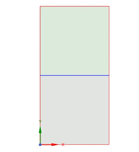
   This is 2D simulation so we create the two square of size 20X20mm one is above the other and we give the name of top square is water and bottom square is air. and use share topology due to that the interface edge is shared .The created geometry is shown below:

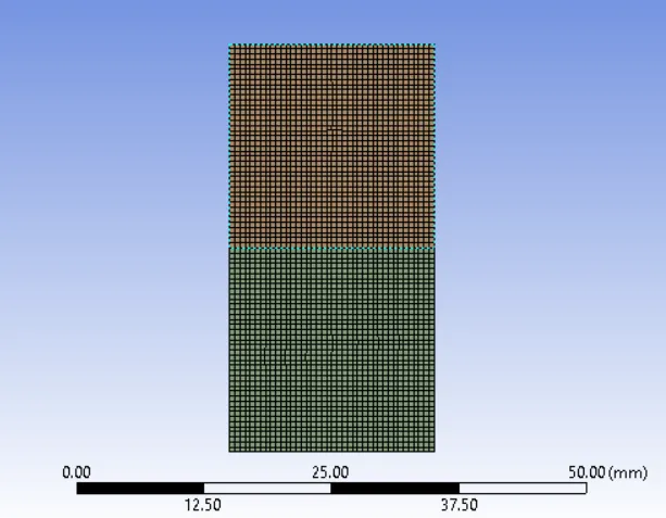
Step 2) Mesh : Use mesh size 0.5 mm 

The mesh is shown below :

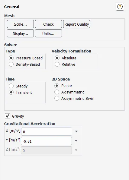
Step 3) Setup and solution:

 

Viscous model: Laminar 

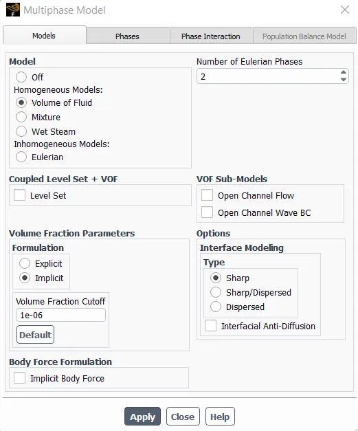
Material : Selected Air and water 

Phase selections :

 

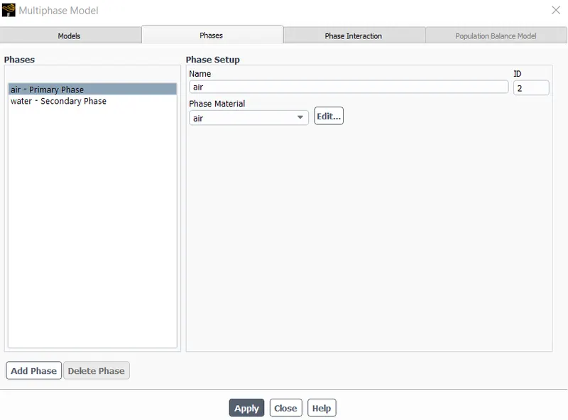
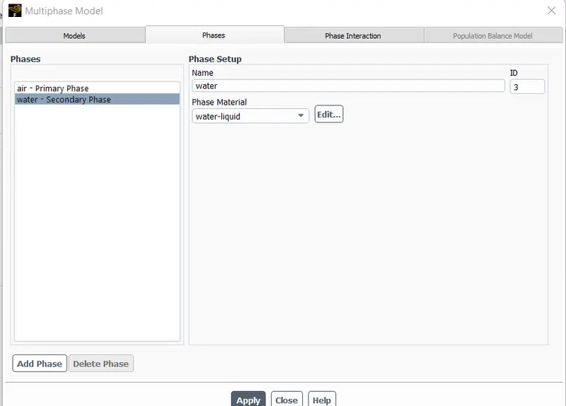
Method of initialization: Standard 

After initialization we required to patch the two phases of the fluid :

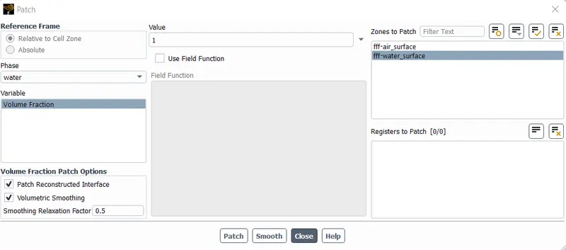
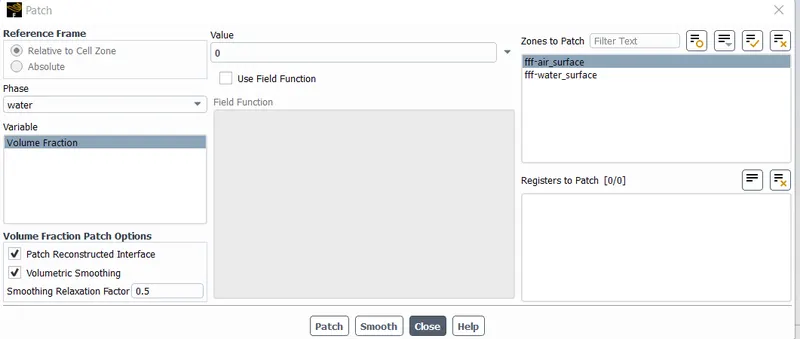
Create a contour :

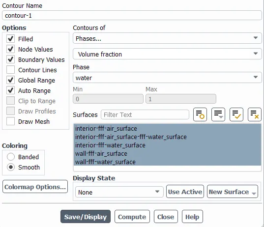
By using contour we create the animation of every time step :

Time step size (sec)= 0.005

No of Time step : 1000 

Result:

Residual plot:

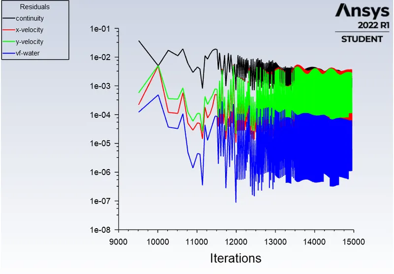
Animation Link: Mesh size : 0.5mm
https://drive.google.com/file/d/1_1BL_PrIlQLxNXl5uVlVoH1bNQevdvxM/view?usp=sharing

Case 2) Mesh size: 0.3 mm

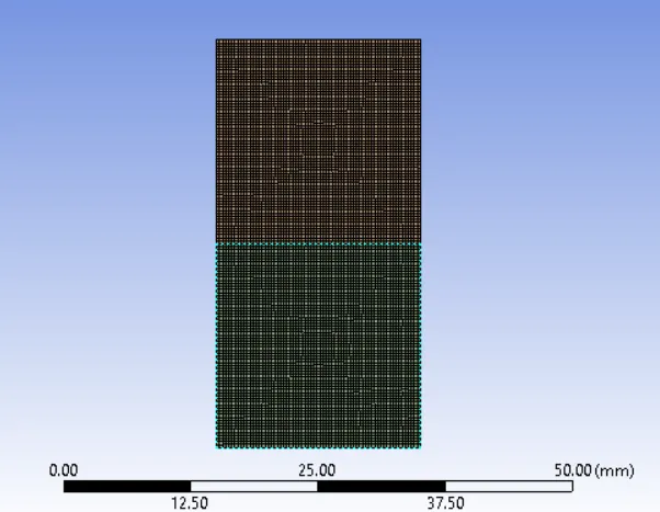
Time step size (sec)= 0.005

No of Time steps : 800 

Result:

Residual plot:

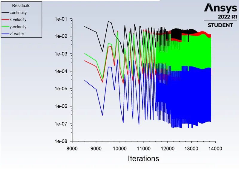
Animation Link: Mesh size : 0.3mm

https://drive.google.com/file/d/1bA_wIRBqIrxDpWjPJneOVqB2FsS8st5a/view?usp=sharing

Case 3) Mesh size: 0.2 mm

 

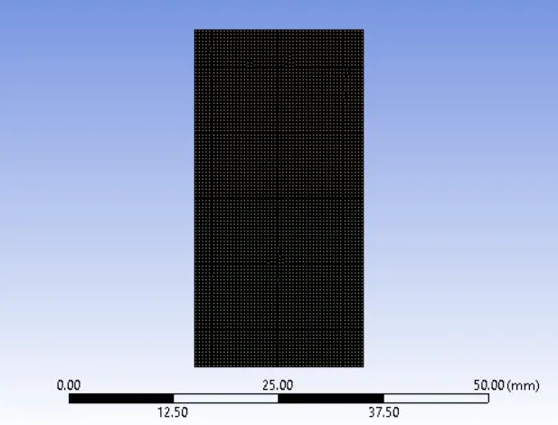
 Time step size (sec)= 0.005

 No of Time steps : 800

Result:

Residual plot:

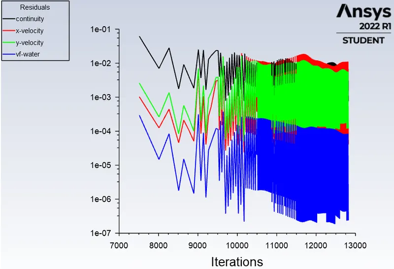
Animation Link: Mesh size : 0.2mm

https://drive.google.com/file/d/1_BcHjdlMswpe2TJldzLfHpI8LoKZp3Jd/view?usp=sharing

Case 4) Run the simulation with water and user-defined material(density = 400 kg/m³, viscosity = 0.001 kg/m-s) for refined mesh. ie Mesh size =0.2mm 

 Time step size (sec)= 0.005

 No of Time steps : 800

Result :

Residual plot:

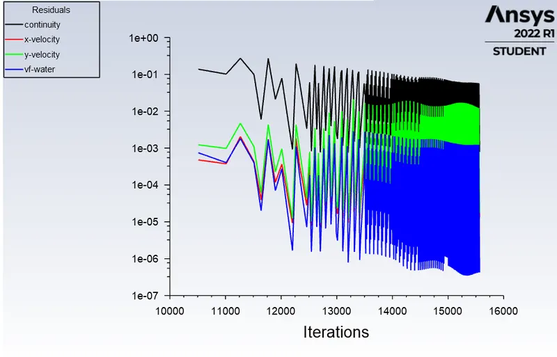
Animation Link: Mesh size : 0.2mm (water-UD material)

https://drive.google.com/file/d/1u_t7yQlF1sCrOeukMC5CbvctWw2UnRNQ/view?usp=sharing

Observations :

• The finer mesh captures the instability better than the coarse mesh.but it takes more time for the heavier fluid to settle down.
• The computational time is also increased for fine mesh but the result obtained having better accuracy.
• The steady state simulation is performed if we are concerned more about the final state results or the equilibrium state,In RT instability CFD model we are more concerned to learn about the transition of the irregularities that start developing when we pour the high densiy fluid upon the low density fluid under the effect of gravity.and we want to know how the interface collapses as a function of time so In this case Transient state is more suitable over the steady state.

Atwood Number:

It is a dimensionless number that is used to study hydrodynamic instabilities  in density stratified flows.

It is denoted by letter A

  `A=(rho_1-rho_2)/(rho_1+rho_2)`      `rarr 1`

where,

`rho_1`=Density of heavier fluid `

`rho_2`=Density of lighter fluid

Calculate the Atwood Number for Air-water RT instability

`rho_1`=998.2 `(kg)/(m^3)` (water density)

`rho_2`=1.225  `(kg)/(m^3)` (Air density)

put this value in equation 1 we get A=0.9975 

Calculate the Atwood Number for Water-UD material RT instability

`rho_1=`998.2 `(kg)/(m^3)` (Water density)

`rho_2`=400 `(kg)/(m^3)` (User defined material density)

put this value in equation 1 we get A=0.4278 

The Atwood number close to 1 then the lighter fluid below the heavier fluid which forms a larger bubbles which is less symmetrical and also it occurs very rapidly.

The Atwood number close to 0 then the lighter fluid below the heavier fluid which forms a  bubbles which is relatively symmetrical and the pertubations are linear for larger time.