Week 5.1 - Mid term project - Solving the steady and unsteady 2D heat conduction problem
Aim: To solve the steady and unsteady state 2D heat conduction equation by using the point iterative techniques such as,Jacobi,Gauss-seidel,Successive over-relaxation,for both implicit and explicit schemes using MATLAB.
Given Parameter:(Boundary Condition):
1) Domain is a area is a Unit square.
2) Assume nx=ny=10 [no of points along x direction=no of points along y direction=10]
3)Boundary conditions are
Top Boundary = 600 K
Bottom Boundary = 900 K
Left Boundary = 400 K
Right Boundary = 800 K
4)Apart from the boundary condition, we assume initial temperature for all the remaining nodes is 300k.
5) Various methods are used to solve the equation are given below:
- Various states: Steady and unsteady state condition
- Various schemes such as Jacobi,Gauss-seidel,Successive over-relaxation.
- Various methods to be used in Unsteady state : Implicit and explicit
Procedure:
Theory:
The 3D Transient (Unsteady) heat conduction equation is given as,
`(delT)/(delt)-alpha((del^2T)/(delx^2)+(del^2T)/(dely^2)+(del^2T)/(delz^2))=0`
It can be written as,
`(delT)/(delt)=alpha((del^2T)/(delx^2)+(del^2T)/(dely^2)+(del^2T)/(delz^2))`
Where,
`alpha=`Thermal diffusivity in `m^2/sec`
We solve the above equation for a thin plate ie two dimensional case for that we neglect the term of Z direction and equation becomes
`(delT)/(delt)=alpha((del^2T)/(delx^2)+(del^2T)/(dely^2))`
The transfer of heat energy occure by two conditions:
- Steady State
- Unsteady / Transient state condition
In steady state condition the Temperature with respect to time is constant .
In Unsteady state condition the temperature with respect to the time is changes as the time passes to reach the steady state condition .
Time loop Logic :
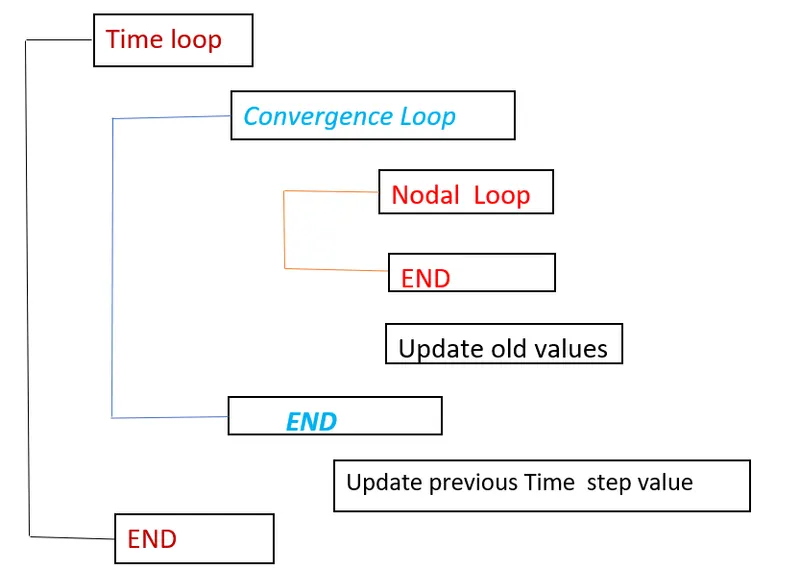
Main program :
There are seven individual program starting from Steady state implicit scheme ,Unsteady state implicit scheme for iterative method such as Jacobi,Gauss-seidel,Successive over-relaxation and followed by Explicit scheme for Unsteady state condition.
Steady State condition (Implicit Scheme):
In steady state condition the Temperature with respect to time is constant so equation for steady state is given as,
`((del^2T)/(delx^2)+(del^2T)/(dely^2))=0`
By discretizing the above equation by applying central difference scheme we get,
`Tp=(1/K).[(T_L+T_R)/(Deltax^2)+(T_T+T_B)/(Deltay^2)]`
here
`K=2((Deltax^2+Deltay^2)/(Deltax^2.Deltay^2))`
but we assume `Deltax=Deltay` so above equation is written as,
`Tp=0.25.(T_L+T_R+T_T+T_B)`
above equation can be written as,
`T_(i,j)=0.25.(T_(i-1,j)+T_(i+1,j)+T_(i,j+1)+T_(i,j-1))`
Matlab code for Steady state equation (method=Jacobi Iteration)
clear all
close all
clc
% Solving the steady state 2D heat conduction equation using Jacobi Method
% Inputs
% No of grid points
nx=10;
ny=nx;

x=linspace(0,1,nx);
dx=x(2)-x(1);
y=linspace(0,1,ny);
dy=dx;

% Absolute error criteria > Tolerance
error=8e9;
tolerance=1e-4;

% Defining boundary conditions
T_L=400;
T_T=600;
T_R=800;
T_B=900;

T=ones([nx,ny])*300;

% Applying the given boundary conditions
T(1,1:nx)=T_T;
T(ny,1:nx)=T_B;
T(2:ny-1,1)=T_L;
T(2:ny-1,nx)=T_R;

% Calculating Average temperature at corners
T(1,1)=(T_T+T_L)/2;
T(nx,ny)=(T_R+T_B)/2;
T(1,ny)=(T_T+T_R)/2;
T(nx,1)=(T_L+T_B)/2;

% Assigning original value to T
T_initial =T;
T_old=T;

% Calculation of 2D steady state heat conduction equation by jacobi method
iterative_solver=1;
if iterative_solver==1
 jacobi_iteration=1;
 while(error>tolerance)

     for i= 2:nx-1
         for j=2:ny-1
             T(i,j)=0.25*((T_old(i,j-1)+T_old(i,j+1)+T_old(i-1,j)+T_old(i+1,j)));
         end
     end
     error=max(max(abs(T_old-T)));
     T_old=T;
     jacobi_iteration=jacobi_iteration+1;
 end
end

% Plotting
figure(1)
contourf(x,y,T)
clabel(contourf(x,y,T))
colorbar
colormap(jet)
set(gca,'ydir','reverse')

xlabel('X-axis')
ylabel('Y-axis')
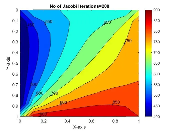
title(sprintf('No of Jacobi Iterations=%d',jacobi_iteration));
pause(0.03);
Explanation of above code is follows:
Step 1) We assume number of grid points along x and y direction of unit square 2D thin plate is 10.
Step 2)For getting linear spaced elements of along x,y direction of unit square domain we use linspace command.
Step 3) We define the Absolute error criteria ie error > tolerance we assume error value 8e9 and given tolerance value is 1e-4. and we define boundary condition and in the inner nodes we assume the temperature is 300K.
Step 4) By using for loop and while loop we calculate temperature value for each iteration and before while loop end we calculate the errror value and update the T_old=T, for using it for next iteration.
Step 5) Plotting,we use contourf command for making contour of Temperature with respect to x and y. and clabel command is used for label the temperature value,colorbar command is used for showing temp.and their color,colormap command is used for showing the different color for different temp. region.
Output :
Matlab code for Steady state equation (method=Gauss Seidel Iteration)
clear all
close all
clc
% Solving the steady state 2D heat conduction equation using Gauss Seidel
% method
% Inputs
% No of grid points
nx=10;
ny=nx;

x=linspace(0,1,nx);
dx=x(2)-x(1);
y=linspace(0,1,ny);
dy=dx;

% Absolute error criteria > Tolerance
error=8e9;
tolerance=1e-4;

% Defining boundary conditions
T_L=400;
T_T=600;
T_R=800;
T_B=900;

T=ones([nx,ny])*300;

% Applying the given boundary conditions
T(1,1:nx)=T_T;
T(ny,1:nx)=T_B;
T(2:ny-1,1)=T_L;
T(2:ny-1,nx)=T_R;

% Calculating Average temperature at corners
T(1,1)=(T_T+T_L)/2;
T(nx,ny)=(T_R+T_B)/2;
T(1,ny)=(T_T+T_R)/2;
T(nx,1)=(T_L+T_B)/2;

% Assigning original value to T
T_initial =T;
T_old=T;

% Calculation of 2D steady state heat conduction equation by Gauss seidel method
iterative_solver=2;
if iterative_solver==2
 GS_iteration=1;
 while(error>tolerance)

     for i= 2:nx-1
         for j=2:ny-1
             T(i,j)=0.25*((T(i,j-1)+T_old(i,j+1)+T(i-1,j)+T_old(i+1,j)));
         end
     end
     error=max(max(abs(T_old-T)));
     T_old=T;
     GS_iteration=GS_iteration+1;
 end
end

% Plotting
figure(1)
contourf(x,y,T)
clabel(contourf(x,y,T))
colorbar
colormap(jet)
set(gca,'ydir','reverse')

xlabel('X-axis')
ylabel('Y-axis')
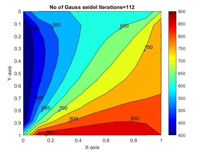
title(sprintf('No of Gauss seidel Iterations=%d',GS_iteration));
pause(0.03);
Output:
Matlab code for Steady state equation (method=Successive over relaxation Iteration)
clear all
close all
clc
% Solving the steady state 2D heat conduction equation using Successive
% over relaxation method
% Inputs
% Number of grid points
nx=10;
ny=nx;

x=linspace(0,1,nx);
dx=x(2)-x(1);
y=linspace(0,1,ny);
dy=dx;

% Absolute error criteria > Tolerance
error=8e9;
tolerance=1e-4;
omega=1.2;

% Defining boundary conditions
T_L=400;
T_T=600;
T_R=800;
T_B=900;

T=ones([nx,ny])*300;

% Applying the given boundary conditions
T(1,1:nx)=T_T;
T(ny,1:nx)=T_B;
T(2:ny-1,1)=T_L;
T(2:ny-1,nx)=T_R;

% Calculating Average temperature at corners
T(1,1)=(T_T+T_L)/2;
T(nx,ny)=(T_R+T_B)/2;
T(1,ny)=(T_T+T_R)/2;
T(nx,1)=(T_L+T_B)/2;

% Assigning original value to T
T_initial =T;
T_old=T;

% Calculation of 2D steady state heat conduction equation by successive over relaxation method
iterative_solver=3;
if iterative_solver==3
 SOR_iteration=1;
 while(error>tolerance)

     for i= 2:nx-1
         for j=2:ny-1
             T(i,j)=(1-omega)*(T_old(i,j))+(omega)*(0.25*((T(i,j-1)+T_old(i,j+1)+T(i-1,j)+T_old(i+1,j))));
         end
      end
     error=max(max(abs(T_old-T)));
     T_old=T;
     SOR_iteration=SOR_iteration+1;
 end
end

% Plotting
figure(1)
contourf(x,y,T)
clabel(contourf(x,y,T))
colorbar
colormap(jet)
set(gca,'ydir','reverse')

xlabel('X-axis')
ylabel('Y-axis')
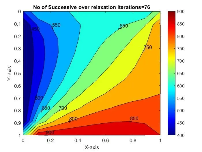
title(sprintf('No of Successive over relaxation iterations=%d',SOR_iteration));
pause(0.03);
Output:
Implicit Scheme Unsteady/Transient state condition:
Unsteady State Equation:
In unsteady state condition the temperature with respect to the time is changes and the system get in steady state after some period.
The equation for Unsteady state is given as,
`(delT)/(delt)=alpha((del^2T)/(delx^2)+(del^2T)/(dely^2))`
We discretize the above equation we get,
`(T_p^(n+1)-T_p^n)/(Deltat)=alpha.((T_L-2T_p+T_R)/(Deltax^2)+(T_T-2T_p+T_B)/(Deltay^2))`
after simplification we get,
`(T_p^(n+1))=1/(1+2K_1+2K_2).(T_P^n+K_1[T_L^(n+1)+T_R^(n+1)]+K_2[T_T^(n+1)+T_B^(n+1)]`
where `K_1=alpha.(Deltat)/(Deltax^2)`, `K_2=alpha.(Deltat)/(Deltay^2)`
`alpha=`Thermal Diffusivity
for better understanding of code
`(T_(i,j)^())=1/(1+2K_1+2K_2).(T_(i,j)^n+K_1[T_(i-1,j)^()+T_(i+1,j^()]]+K_2[T_(i,j+1)+T_(i,j-1)^()])`
Matlab code for solving Unsteady State equation Implicit Scheme [Method= Jacobi Iteration]
clear all
close all
clc
% Solving the Unsteady state 2D heat conduction equation using Jacobi Method
% Inputs
% No of grid points
nx=10;
ny=nx;
nt=1400;
alpha=1.1;

x=linspace(0,1,nx);
dx=x(2)-x(1);
y=linspace(0,1,ny);
dy=dx;

% Absolute error criteria > Tolerance
error=8e9;
tolerance=1e-4;
dt=1e-3;

% Defining boundary conditions
T_L=400;
T_T=600;
T_R=800;
T_B=900;

T=ones([nx,ny])*300;

T(1,1:nx)=T_T;
T(ny,1:nx)=T_B;
T(2:ny-1,1)=T_L;
T(2:ny-1,nx)=T_R;

% Calculating Average temperature at corners
T(1,1)=(T_T+T_L)/2;
T(nx,ny)=(T_R+T_B)/2;
T(1,ny)=(T_T+T_R)/2;
T(nx,1)=(T_L+T_B)/2;

% Assigning original value to T
T_initial =T;
T_old=T;

%Calculation of Unsteady state 2D heat conduction equation using Jacobi Method
k1= alpha*(dt/(dx^2));
k2= alpha*(dt/(dy^2));

jacobi_iteration=1;
for k=1:nt
    error= 8e9;
    while(error>tolerance)

     for i= 2:nx-1
         for j=2:ny-1
             Term_1= 1/(1+(2*k1)+(2*k2));
             Term_2=k1*Term_1;
             Term_3=k2*Term_1;
             H=(T_old(i-1,j))+(T_old(i+1,j));
             V=(T_old(i,j+1))+(T_old(i,j-1));

             T(i,j)=(T_initial(i,j)*Term_1)+(H*Term_2)+(V*Term_3);

         end
     end
      error=max(max(abs(T_old-T)));
     T_old=T;
     jacobi_iteration=jacobi_iteration+1;
    end
T_initial=T;
figure(1)
contourf(x,y,T)
clabel(contourf(x,y,T))
colorbar
colormap(jet)
set(gca,'ydir','reverse')

xlabel('X-axis')
ylabel('Y-axis')
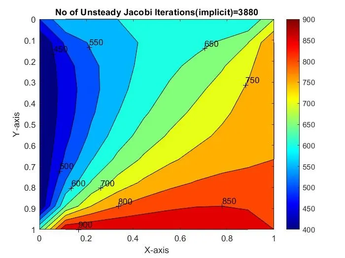
title(sprintf('No of Unsteady Jacobi Iterations(implicit)=%d',jacobi_iteration));
pause(0.03);
end
Output:
Matlab code for solving Unsteady State equation Implicit Scheme [Method= Gauss Seidel Iteration]
clear all
close all
clc
% Solving the Unsteady state 2D heat conduction equation using Gauss Seidel Method
% Inputs
% No of grid points
nx=10;
ny=nx;
nt=1400;
alpha=1.1;

x=linspace(0,1,nx);
dx=x(2)-x(1);
y=linspace(0,1,ny);
dy=dx;

% Absolute error criteria > Tolerance
error=8e9;
tolerance=1e-4;
dt=1e-3;

% Defining boundary conditions
T_L=400;
T_T=600;
T_R=800;
T_B=900;

T=ones([nx,ny])*300;

T(1,1:nx)=T_T;
T(ny,1:nx)=T_B;
T(2:ny-1,1)=T_L;
T(2:ny-1,nx)=T_R;

% Calculating Average temperature at corners
T(1,1)=(T_T+T_L)/2;
T(nx,ny)=(T_R+T_B)/2;
T(1,ny)=(T_T+T_R)/2;
T(nx,1)=(T_L+T_B)/2;

% Assigning original value to T
T_initial =T;
T_old=T;

%Calculation of Unsteady state 2D heat conduction equation using Gauss Seidel Method
k1= alpha*(dt/(dx^2));
k2= alpha*(dt/(dy^2));

GS_iteration=1;
for k=1:nt
    error= 8e9;
    while(error>tolerance)

     for i= 2:nx-1
         for j=2:ny-1
             Term_1= 1/(1+(2*k1)+(2*k2));
             Term_2=k1*Term_1;
             Term_3=k2*Term_1;
             H=(T(i-1,j))+(T_old(i+1,j));
             V=(T(i,j+1))+(T_old(i,j-1));

             T(i,j)=(T_initial(i,j)*Term_1)+(H*Term_2)+(V*Term_3);

         end
     end
      error=max(max(abs(T_old-T)));
     T_old=T;
     GS_iteration=GS_iteration+1;
    end
T_initial=T;
% Plotting
figure(1)
contourf(x,y,T)
clabel(contourf(x,y,T))
colorbar
colormap(jet)
set(gca,'ydir','reverse')

xlabel('X-axis')
ylabel('Y-axis')
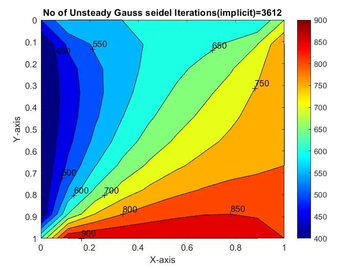
title(sprintf('No of Unsteady Gauss seidel Iterations(implicit)=%d',GS_iteration));
pause(0.03);
end
Output:
Matlab code for solving Unsteady State equation Implicit Scheme [Method= Successive over relaxation Iteration]
clear all
close all
clc
% Solving the Unsteady state 2D heat conduction equation using Successive over relaxation Method
% Inputs
% No of grid points
nx=10;
ny=nx;
nt=1400;
alpha=1.1;

x=linspace(0,1,nx);
dx=x(2)-x(1);
y=linspace(0,1,ny);
dy=dx;

% Absolute error criteria > Tolerance
error=8e9;
tolerance=1e-4;
dt=1e-3;
omega= 1.1 ;
% Defining boundary conditions
T_L=400;
T_T=600;
T_R=800;
T_B=900;

T=ones([nx,ny])*300;

T(1,1:nx)=T_T;
T(ny,1:nx)=T_B;
T(2:ny-1,1)=T_L;
T(2:ny-1,nx)=T_R;

% Calculating Average temperature at corners
T(1,1)=(T_T+T_L)/2;
T(nx,ny)=(T_R+T_B)/2;
T(1,ny)=(T_T+T_R)/2;
T(nx,1)=(T_L+T_B)/2;

% Assigning original value to T
T_initial =T;
T_old=T;
T_end=T;

%Calculation of Unsteady state 2D heat conduction equation using Successive over relaxation Method
k1= alpha*(dt/(dx^2));
k2= alpha*(dt/(dy^2));

SOR_iteration=1;
for k=1:nt
    error= 8e9;
    while(error>tolerance)

     for i= 2:nx-1
         for j=2:ny-1
             Term_1= 1/(1+(2*k1)+(2*k2));
             Term_2=k1*Term_1;
             Term_3=k2*Term_1;
             H=(T(i-1,j))+(T_old(i+1,j));
             V=(T(i,j+1))+(T_old(i,j-1));

             T(i,j)=(T_initial(i,j)*Term_1)+(H*Term_2)+(V*Term_3);
             T_end(i,j)=((1-omega)*T_old(i,j))+(T(i,j)*omega);

         end
     end
      error=max(max(abs(T_old-T)));
     T_old=T_end;
     SOR_iteration=SOR_iteration+1;
    end
T_initial=T_end;
%Plotting
figure(1)
contourf(x,y,T)
clabel(contourf(x,y,T))
colorbar
colormap(jet)
set(gca,'ydir','reverse')

xlabel('X-axis')
ylabel('Y-axis')
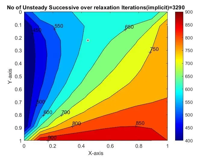
title(sprintf('No of Unsteady Successive over relaxation Iterations(implicit)=%d',SOR_iteration));
pause(0.03);
end
Output:
Explicit Scheme Unsteady/Transient state condition:
Unsteady State Equation:
The equation for Unsteady state is given as,
`(delT)/(delt)=alpha((del^2T)/(delx^2)+(del^2T)/(dely^2))`
If we discretize above equation we get,
`(T_p^(n+1)-T_p^n)/(Deltat)=alpha.((T_L-2T_p+T_R)/(Deltax^2)+(T_T-2T_p+T_B)/(Deltay^2))`
If we simplify the above equation,
`(T_p^(n+1))=T_p^n+K_1(T_L-2T_p+T_R)^n+K_2(T_T-2T_p+T_B)^n`
where `K_1=alpha.(Deltat)/(Deltax^2)`, `K_2=alpha.(Deltat)/(Deltay^2)`
For the better understanding for code, we can write,
`(T_(i,j)^())=T_(i,j)+K_1(T_(i-1,j)-2T_(i,j)+T_(i+1,j))+K_2(T_(i,j+1)-2T_(i,j)+T_(i,j-1))`
Matlab code for solving Unsteady State equation Explicit Scheme :
clear all
close all
clc
% Solving the Unsteady state 2D heat conduction equation (Explicit scheme)
% Inputs
% No of grid points
nx=10;
ny=nx;
nt=1400;
alpha=1.1;


x=linspace(0,1,nx);
dx=x(2)-x(1);
y=linspace(0,1,ny);
dy=dx;

% Absolute error criteria > Tolerance
error=8e9;
tolerance=1e-4;
dt=1e-3;

% Defining boundary conditions
T_L=400;
T_T=600;
T_R=800;
T_B=900;

T=ones([nx,ny])*300;

T(1,1:nx)=T_T;
T(ny,1:nx)=T_B;
T(2:ny-1,1)=T_L;
T(2:ny-1,nx)=T_R;

% Calculating Average temperature at corners
T(1,1)=(T_T+T_L)/2;
T(nx,ny)=(T_R+T_B)/2;
T(1,ny)=(T_T+T_R)/2;
T(nx,1)=(T_L+T_B)/2;

% Assigning original value to T
T_initial =T;
T_old=T;


%Calculation of Unsteady state 2D heat conduction equation using Explicit
%scheme
k1= alpha*(dt/(dx^2));
k2= alpha*(dt/(dy^2));
iterative_solver=1;
if iterative_solver ==1
    Unsteady_Explicit = 1;
 for k=1:nt
    error= 8e9;
    while(error>tolerance)

     for i= 2:nx-1
         for j=2:ny-1
             Term_1= T_old(i,j);
             Term_2=k1*(T_old(i+1,j)-2*T_old(i,j)+T_old(i-1,j));
             Term_3=k2*(T_old(i,j+1)-2*T_old(i,j)+T_old(i,j-1));

             T(i,j)=Term_1+Term_2+Term_3;

         end
     end
      error=max(max(abs(T_old-T)));
     T_old=T;
     Unsteady_Explicit=Unsteady_Explicit+1;
    end
 end
end

%Plotting
figure(1)
contourf(x,y,T)
clabel(contourf(x,y,T))
colorbar
colormap(jet)
set(gca,'ydir','reverse')

xlabel('X-axis')
ylabel('Y-axis')
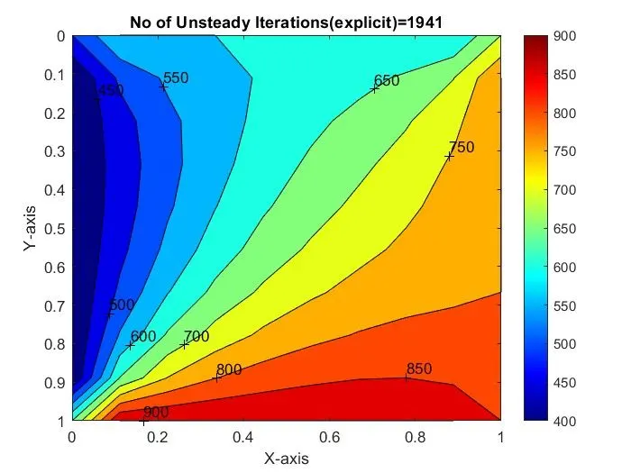
title(sprintf('No of Unsteady Iterations(explicit)=%d',Unsteady_Explicit));
pause(0.03);
Output:
Conclusion:
| Types of Scheme | Methods of Iteration | No of Iterations |
| Implicit -Steady state Analysis | Jacobi | 208 |
| Gauss Seidel | 112 | |
| Successive over relaxation | 76 | |
| Implicit -UnSteady state Analysis | Jacobi | 3880 |
| Gauss Seidel | 3612 | |
| Successive over relaxation | 3290 | |
| Explicit- UnSteady state Analysis | 1941 |
From the outputs of above various methods and there no of Iterations we can conclude that,
- Jacobi>Gauss seidel>Successive over relaxation According to the number of iteration calculated for all the methods and schemes.
- When comparing the steady state and Unsteady state,It is proved that steady state takes less time for execution and it gives result in least number of iterations.
- SOR Iteration method is the most effective iteration method because it tooks less number of iteration for converging the solution in both implicit and explicit scheme compared to Jacobi and gauss seidel.