Mixing Efficiency Of A Mixing Tee.(ANSYS FLUENT)

AIM:

To understand a mixing tee and carry out various simulations under different initial conditions and understand its effectiveness.

OBJECTIVE:

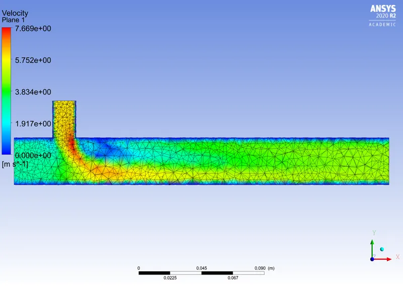
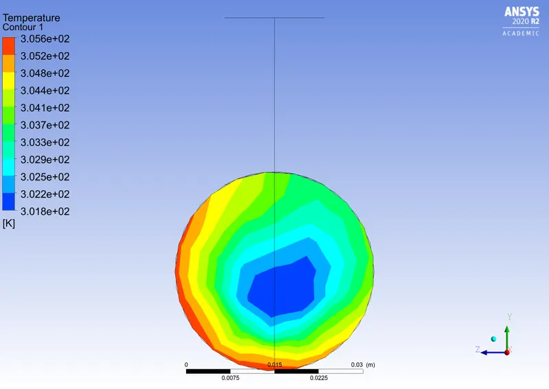
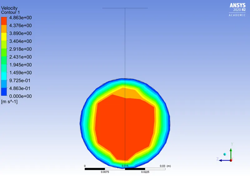
1. Plot Velocity and temperature contour plots on the cut planes along and across the pipe.
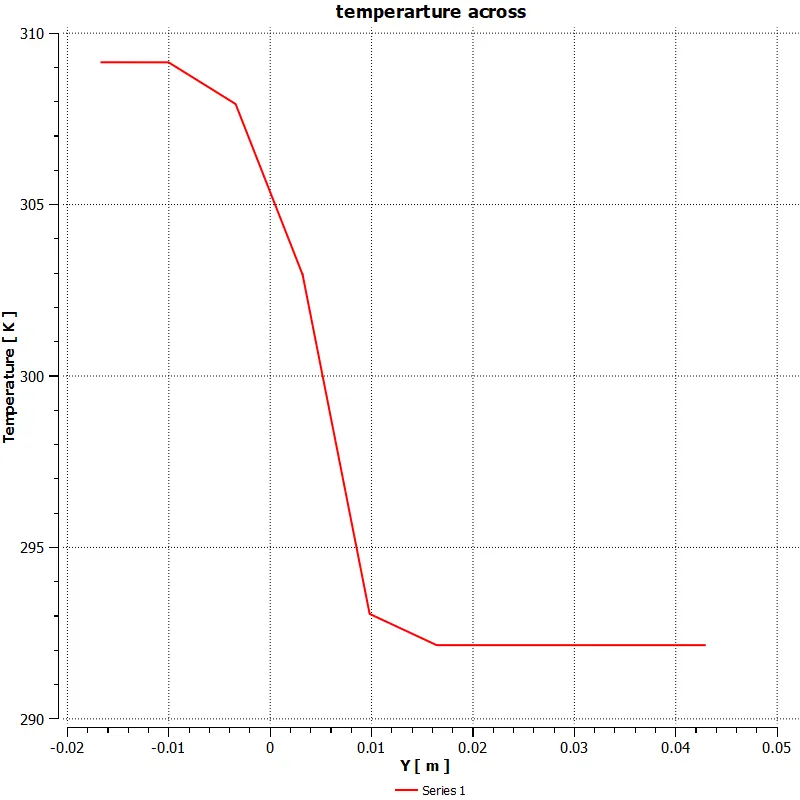
2. Plot Velocity and temperature line plots along and across the length of the pipe.
3. Perform Mesh independent study for any one case.
4. Discuss the effect of length and momentum ratio on results.
5. make a table comparing the values of cell count,avg outlet temperature and number of iterations for convergence.

THEORY:

Mixing Tee: a mixing tee is a device used in various chemical diffusion/ mixing processes in devices such as an air conditioner for mixing the fresh air and the return air. we can varry various parameters such as temperature by changing the velocity of the fluid entering into the mixing tee. In this project we conduct various steady state simulations for a 'short' and 'long' mixing tee, with different momentum ratios, to understand its working.

TURBULENCE:

In fluid dynamics, turbulence or turbulent flow is fluid motion characterized by chaotic changes in pressure and flow velocity. It is in contrast to a laminar flow, which occurs when a fluid flows in parallel layers, with no disruption between those layers.

Turbulence is commonly observed in everyday phenomena such as surf, fast flowing rivers, billowing storm clouds, or smoke from a chimney, and most fluid flows occurring in nature or created in engineering applications are turbulent. Turbulence is caused by excessive kinetic energy in parts of a fluid flow, which overcomes the damping effect of the fluid's viscosity. For this reason turbulence is commonly realized in low viscosity fluids. In general terms, in turbulent flow, unsteady vortices appear of many sizes which interact with each other, consequently drag due to friction effects increases. This increases the energy needed to pump fluid through a pipe.

in general fluid flows turbulence is the norm and laminar flow is the exception. turbulence is a very complicated phenomenon, our understanding of which is very limited. thus when we try to model turbulence in a simulation there are various approaches that exist. it is on us to select a approach that works well with the physics of the problem.

CONVERGENCE:

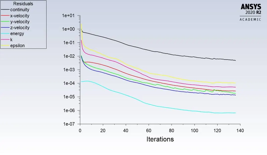
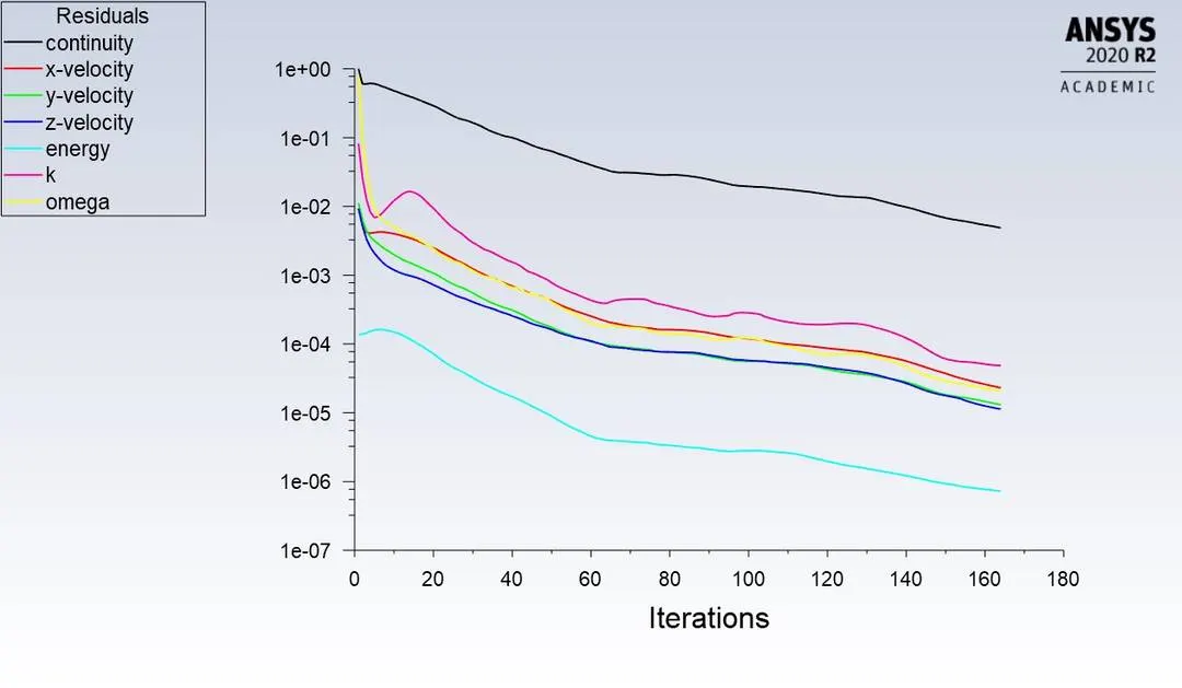
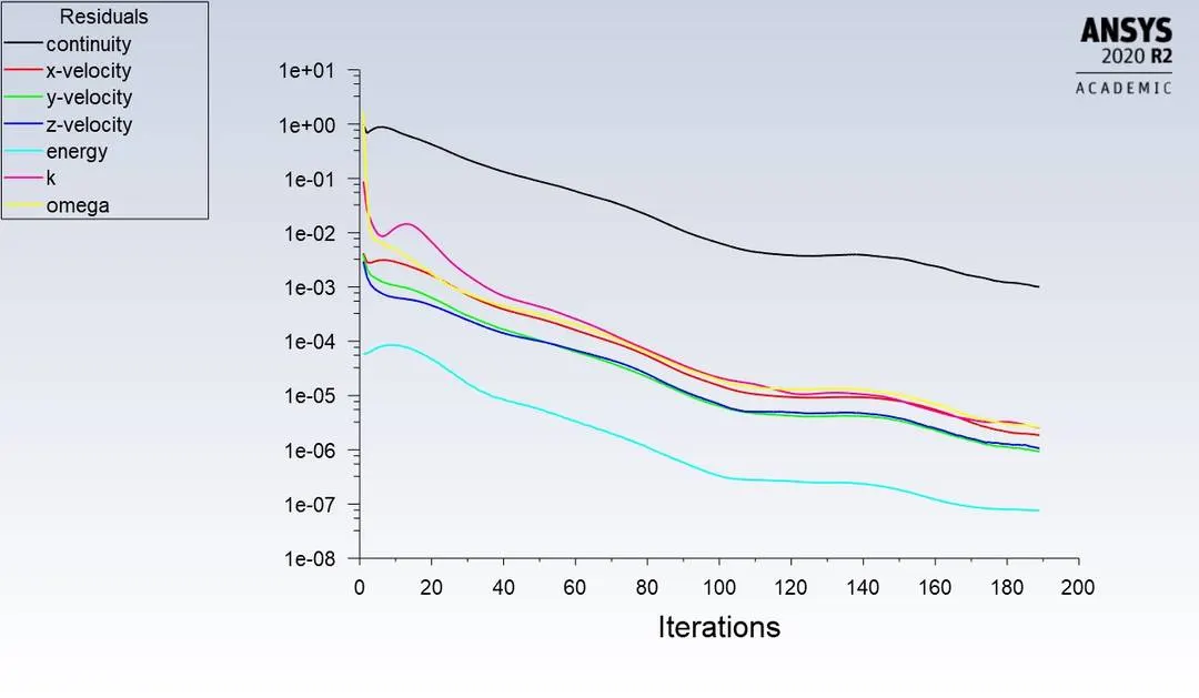
Since most fluid flow problems are of a non- linear nature, dealing with phenomenon like turbulence. to solve such problems we use an iterative solver to continuously improve our solution till 'convergence ' is reached. when solving a problem with multiple iterations convergence becomes related to the accuracy of the solution. typically when assessing convergence for a steady-state CFD solution we need to keep in mind three major things, they are:

1. Residual values
2. Solution Imbalance
3. Observing quantities of interest

the criteria for convergence that is being applied is:

1. continuity
2. x- velocty
3. y- velocity
4. z-velocity
5. energy
6. turbulence related variable

Y+:

y+ is a non dimensional term that is used to define how fine or course the mesh is, This helps us determine if we need to use specific wall function.

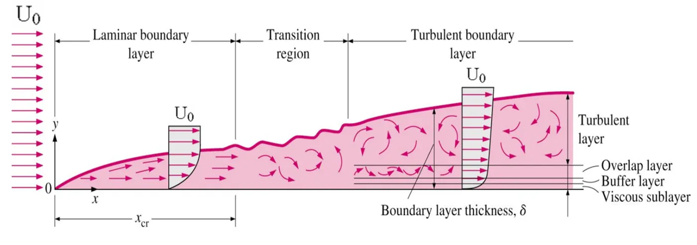
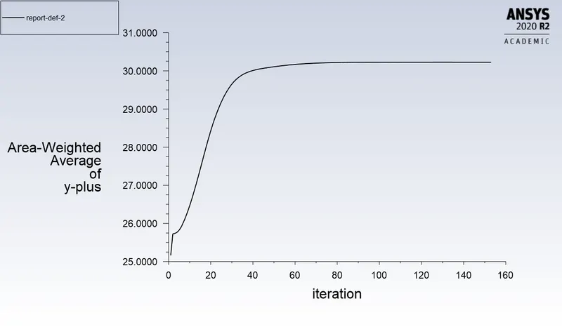
when we consider a boundary layer, there exist 2 regions the inner boundary layer and the outer boundary layer. The inner boundary layer consists of 3 main regions, the first is the viscous region which is right after the wall, in this region the viscous forces dominate the interial forces and the flow is laminar(y+ <10). The next is the transition region(10 < y+ < 30 ) and the third is the turbulent boundary layer, here the inertial forces are more dominant(30 < Y+ <300). The y+ value helps us decide the type of turbulence model that we need to use for the perticular problem.

turbulence models:

Reynolds averaged navier stokes equation:

The Reynolds-averaged Navier–Stokes equations (or RANS equations) are time-averaged equations of motion for fluid flow. The idea behind the equations is Reynolds decomposition, whereby an instantaneous quantity is decomposed into its time-averaged and fluctuating quantities.The RANS equations are primarily used to describe turbulent flows. These equations can be used with approximations based on knowledge of the properties of flow turbulence to give approximate time-averaged solutions to the Navier–Stokes equations.

1) k-Epsilon:

K-epsilon (k-ε) turbulence model is the most common model used in Computational Fluid Dynamics (CFD) to simulate mean flow characteristics for turbulent flow conditions. It is a two equation model that gives a general description of turbulence by means of two transport equations (PDEs). The original impetus for the K-epsilon model was to improve the mixing-length model.In the k–ε model the kinematic eddy viscosity νt is expressed as the product of a velocity scale ϑ = k and a length scale l= k3/2/ε. The rate of dissipation of turbulence kinetic energy ε is not the only possible length scale determining variable
Realizable k- ε Model: An immediate benefit of the realizable k-ɛ model is that it provides improved predictions for the spreading rate of both planar and round jets. It also exhibits superior performance for flows involving rotation, boundary layers under strong adverse pressure gradients, separation, and recirculation. In virtually every measure of comparison, Realizable k-ɛ demonstrates a superior ability to capture the mean flow of the complex structures.

2)k- omega:

In computational fluid dynamics, the k–omega (k–ω) turbulence model is a common two-equation turbulence model, that is used as an approximation for the Reynolds-averaged Navier–Stokes equations (RANS equations). The model attempts to predict turbulence by two partial differential equations for two variables, k and ω, with the first variable being the turbulence kinetic energy (k) while the second (ω) is the specific rate of dissipation (of the turbulence kinetic energy k into internal thermal energy).
The k–ω model initially attracted attention because integration to the wall does not require wall-damping functions in low Reynolds number applications. The value of turbulence kinetic energy k at the wall is set to zero. The frequency ω tends to infinity at the wall, but we can specify a very large value at the wall.apply a hyperbolic variation ωP = 6ν/(β1 y^P/2) at the near-wall grid point. Practical experience with the model has shown that the results do not depend too much on the precise details of this treatment.

the results of the k–ε model are much less sensitive to the (arbitrary) assumed values in the free stream, but its near-wall performance is unsatisfactory for boundary layers with adverse pressure gradients. This led to suggest a hybrid model using (i) a transformation of the k–ε model into a k–ω model in the near-wall region and (ii) the standard k–ε model in the fully turbulent region far from the wall, the ε-equation is transformed into an ω-equation by substituting ε = kω. this became the k–ω sst model.

CASE SETUP:

1) The first step to running the simulation is to load the geometry and extracting the volume of the geometry.
2) After extracting the volume we must carry out the meshing of the volume, here we must specify the mesh size.
3) After meshing the component we need to label the surfaces of the volume as inlet, outlet,walls etc.
4) Next we need to go to the setup menu and perform a mesh check, this is done on fluent.
5) we select a pressure based solver, absolute velocity formationand steady state in the general task page.
6) tick the energy box and set up the type of viscous condition as either k-epison (realisible) or k-omega(sst)
7) Next we setup the boundary conditions at the inlet x and y, outlet and the wall conditions
8) change the materials to the desired material in the material box and in the cellzones box.
9) add the plot definitions that we wish to print in the solution tab.
10) initialise the system, and set the number of iterations required.
11) Press calculate to start the simulation.
12) Once the simulation is complete, go to cfd-post to view the results and to plot the graphs.

TABLE:

type	turbulence model	mesh cell size	cell count	weighted average outlet temperature(celcius)	no of iterations
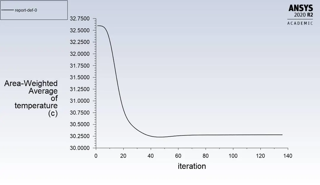
short tee momentum ratio -2	k- episilon	5 mm	14330	30.25	135
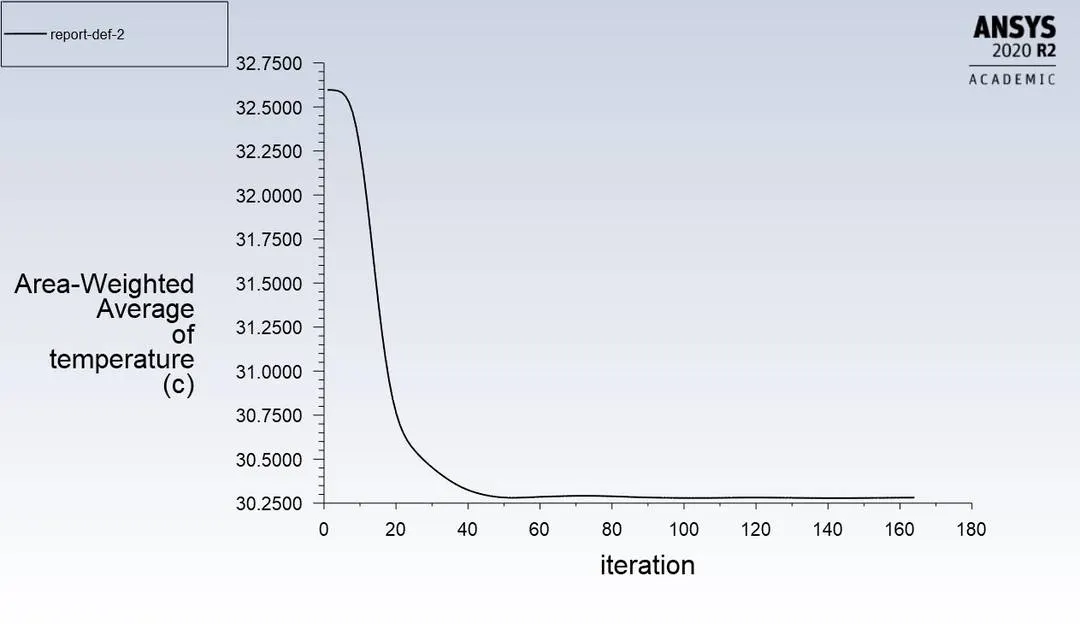
short tee momentum ratio -2	k-omega	5 mm	14330	30.3	165
short tee momentum ratio -2	k-omega	1.5 mm	211968	30.5	190
short tee momentum ratio -2	k-omega	3 mm	39734	30.3	180
short tee momentum ratio -4	k-omega	5 mm	14330	27.5	275
long tee momentum ratio - 2	k-omega	5 mm	18173	30.4	225
long tee momentum ratio - 4	k-omega	5 mm	18173	27.4	150

SOLUTION IMAGES:

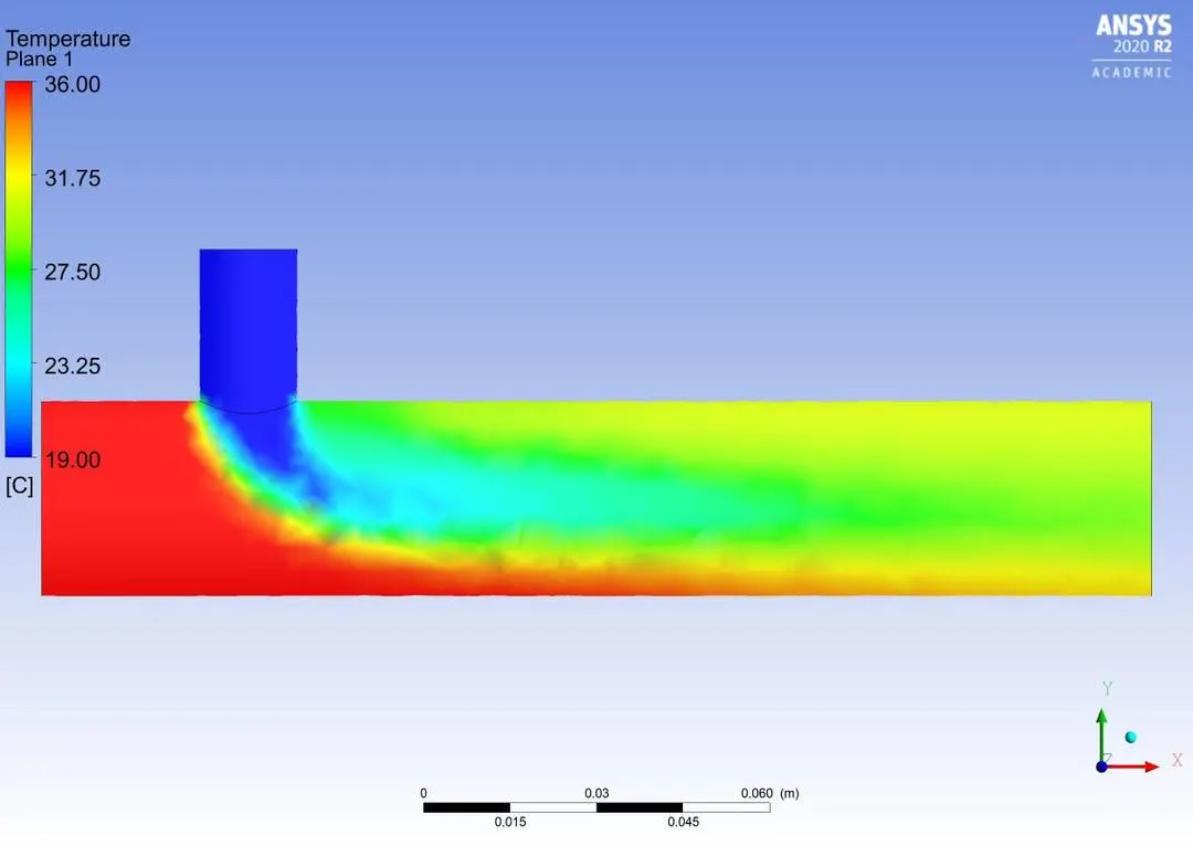
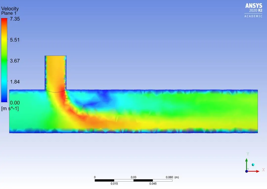
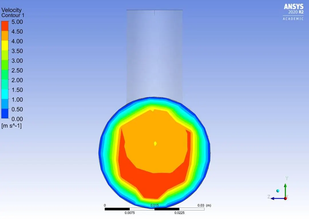
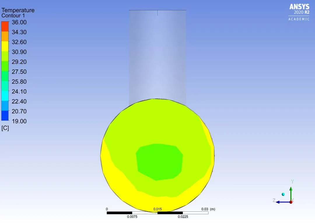
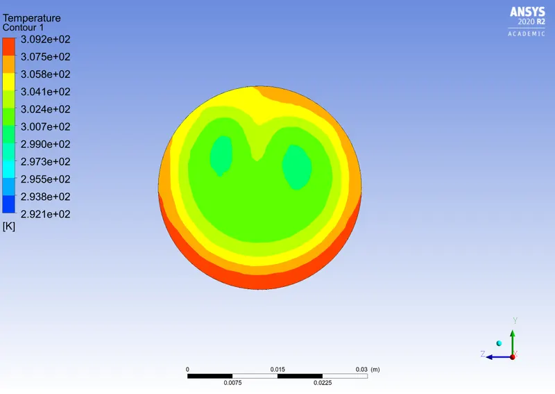
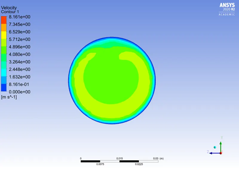
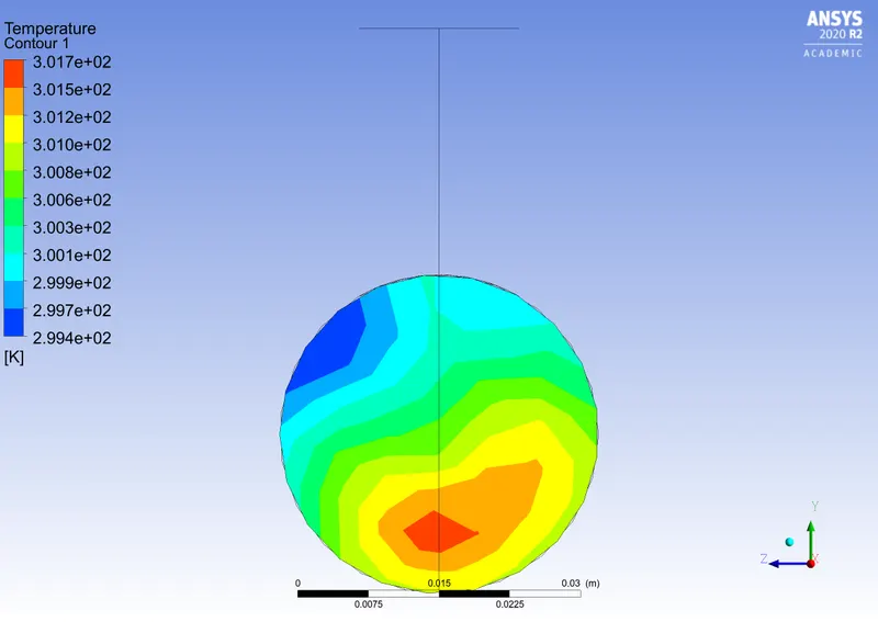
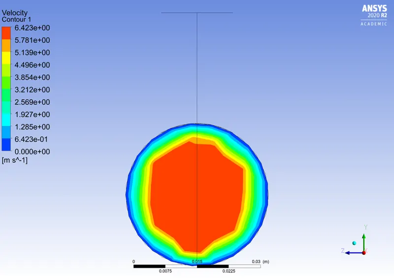
CASE 1: momentum ratio -2; k-epislon solver; mesh size: 5mm; size: short

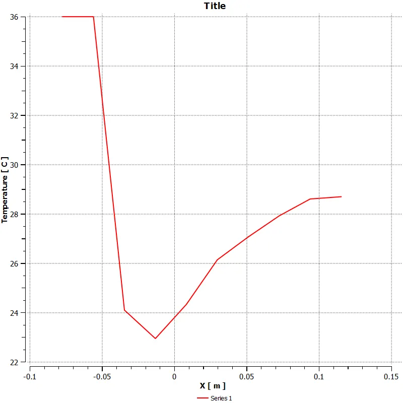
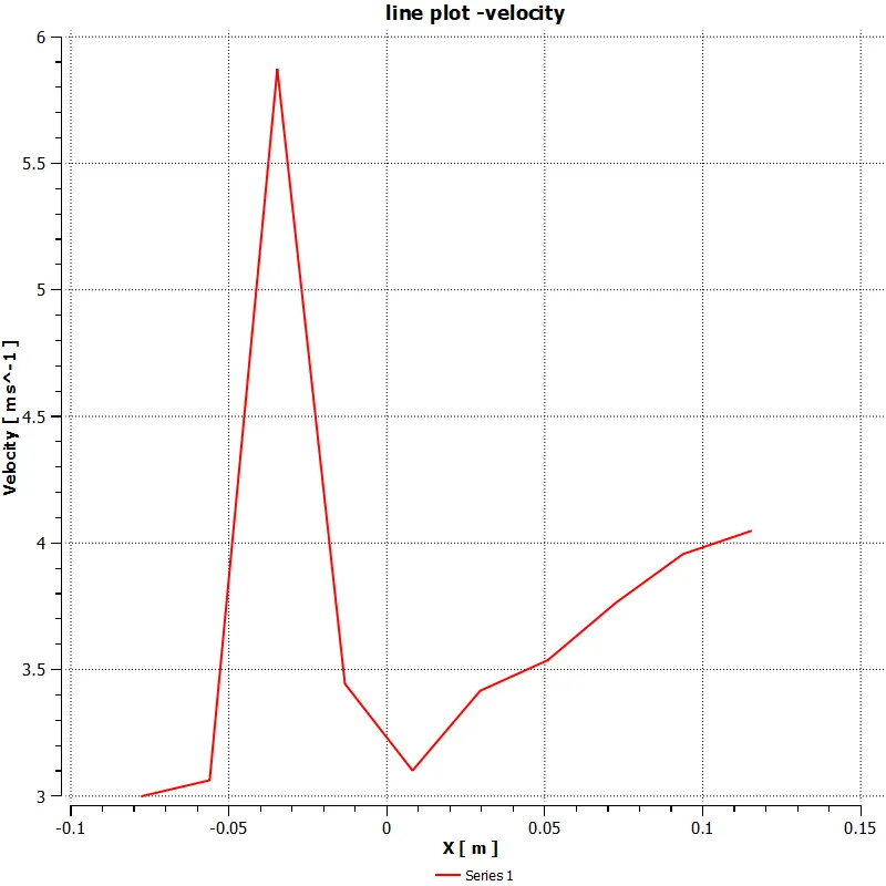
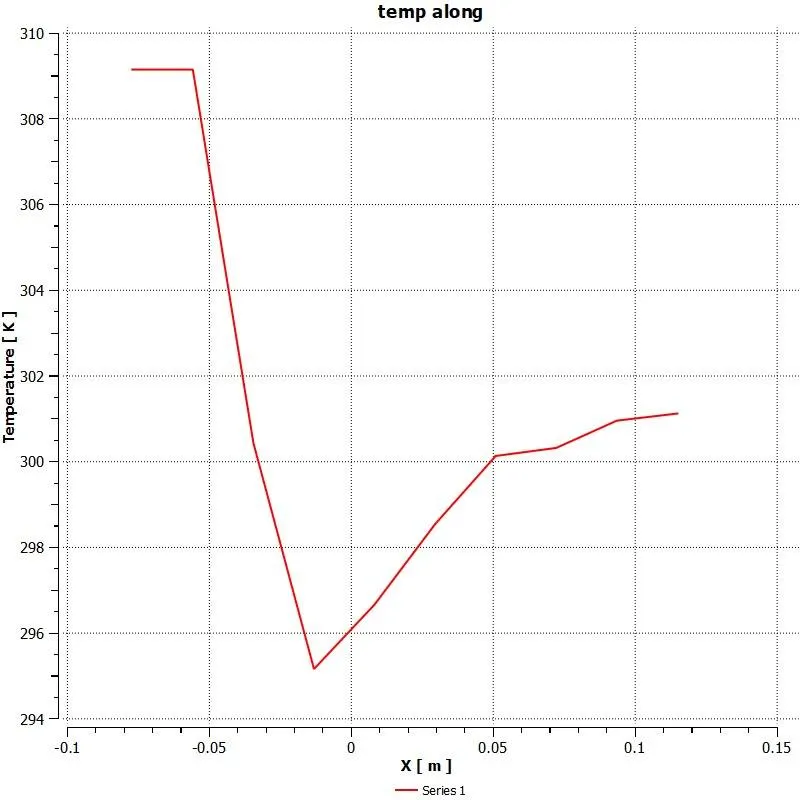
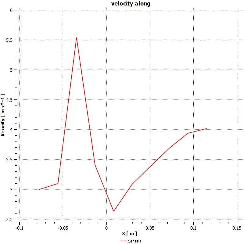
line along plot:

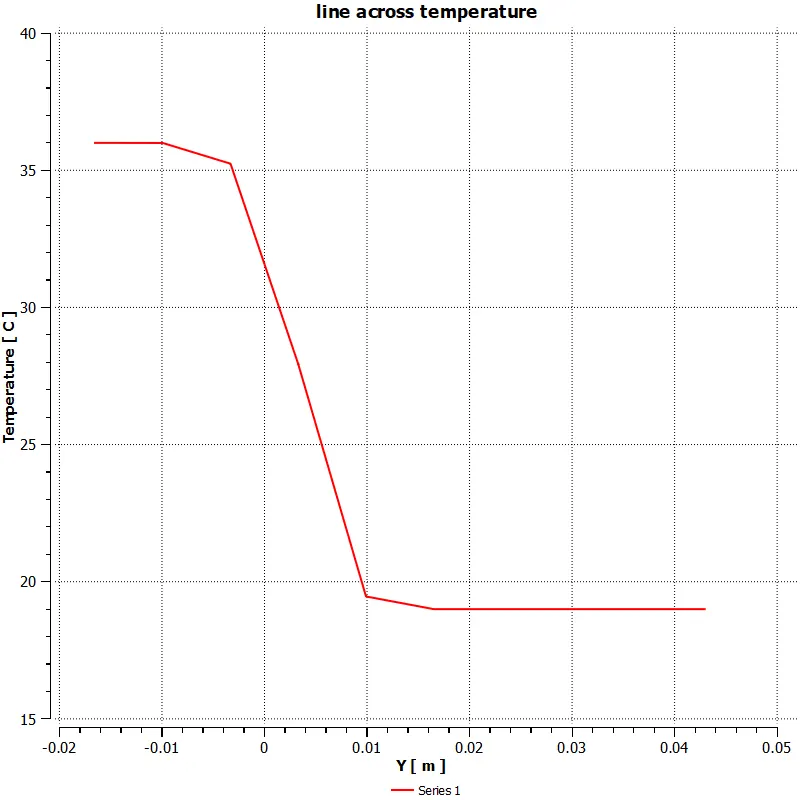
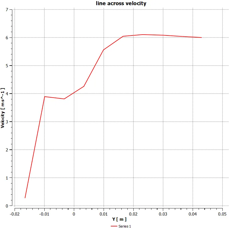
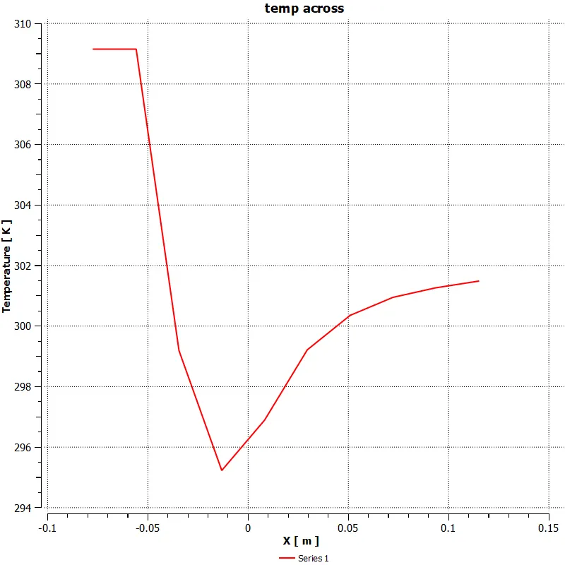
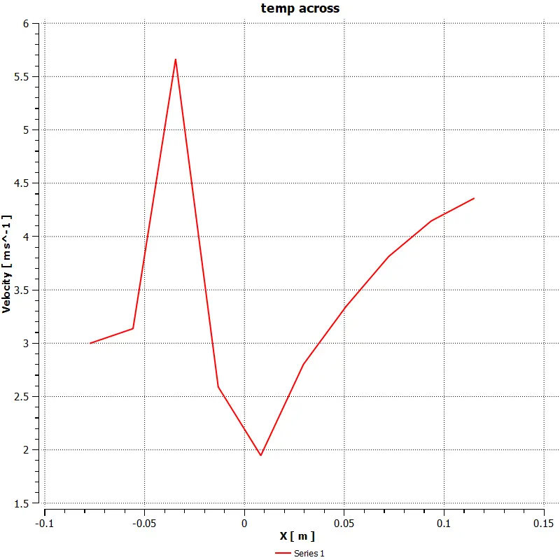
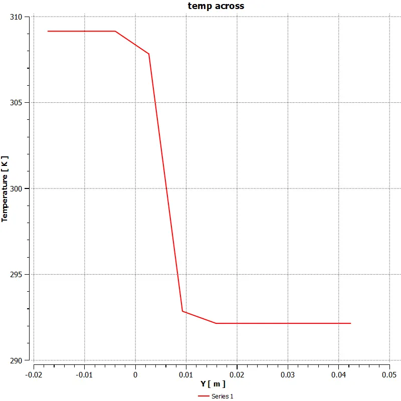
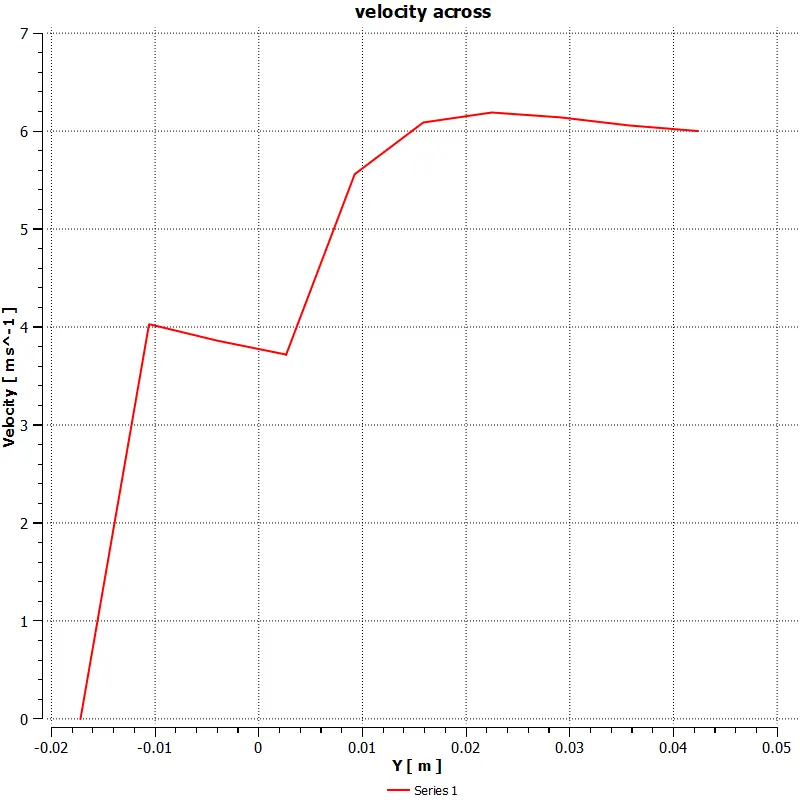
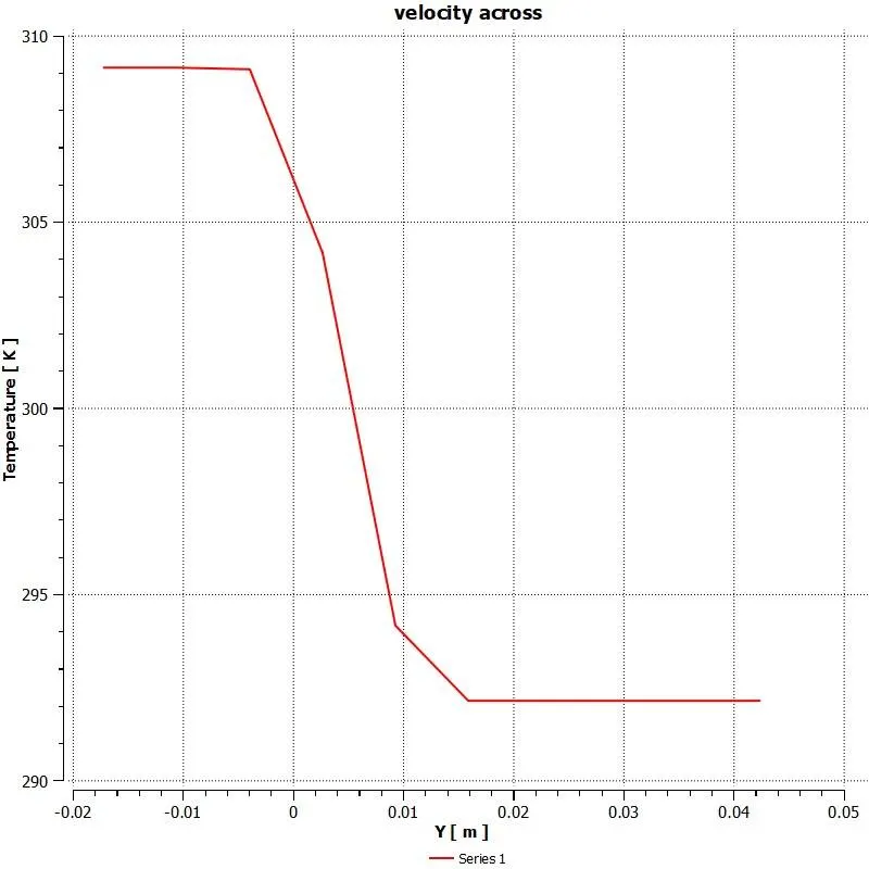
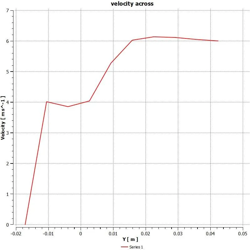
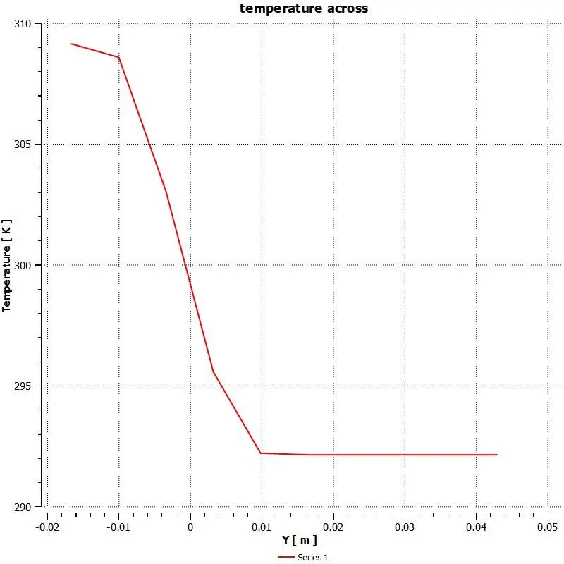
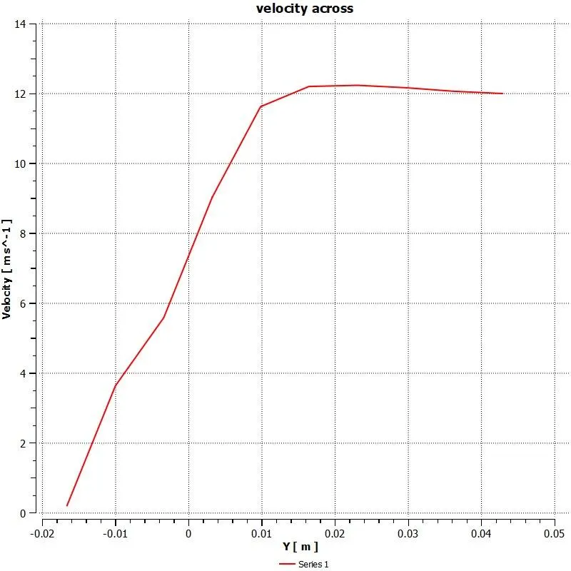
line across plot:

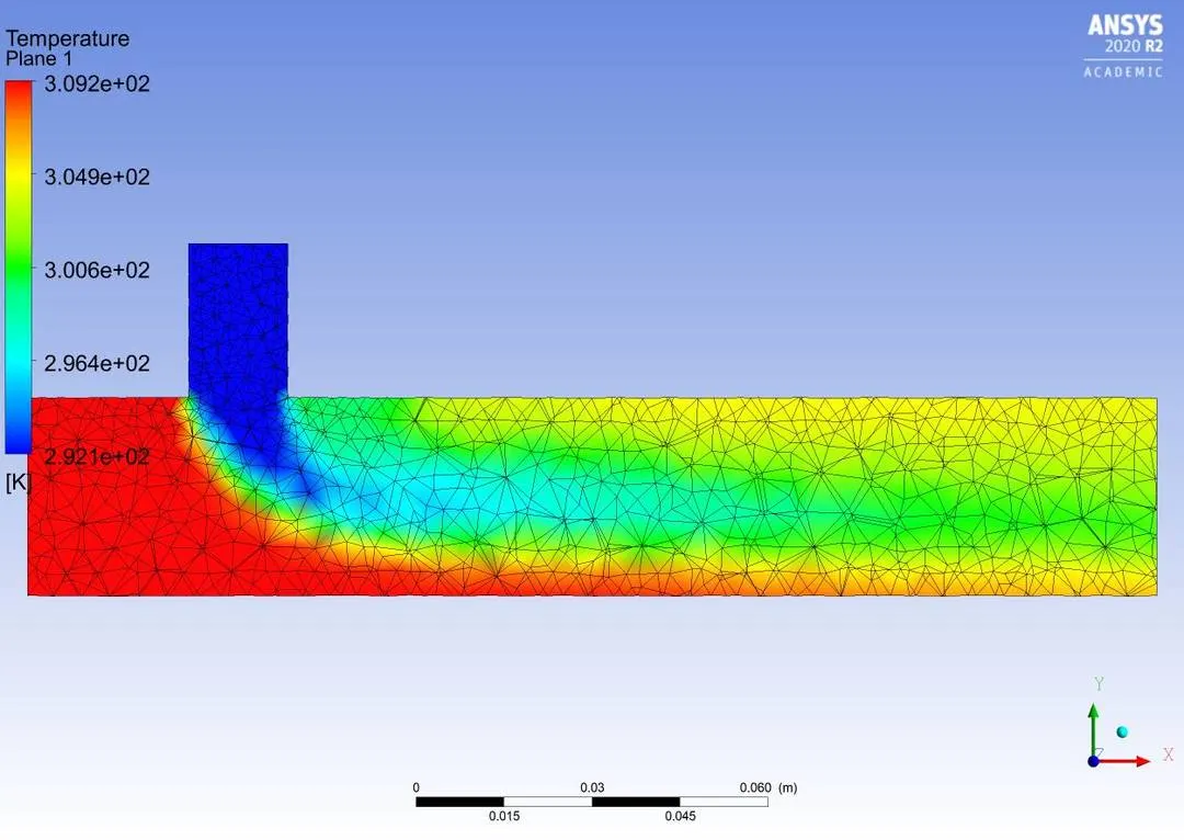
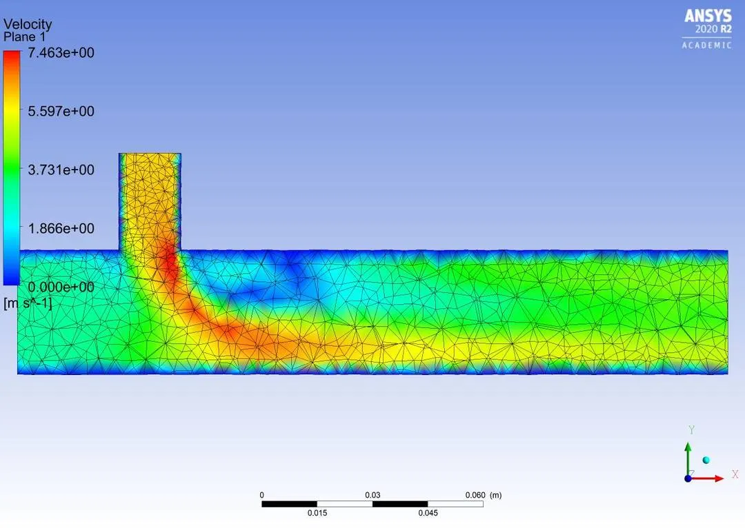
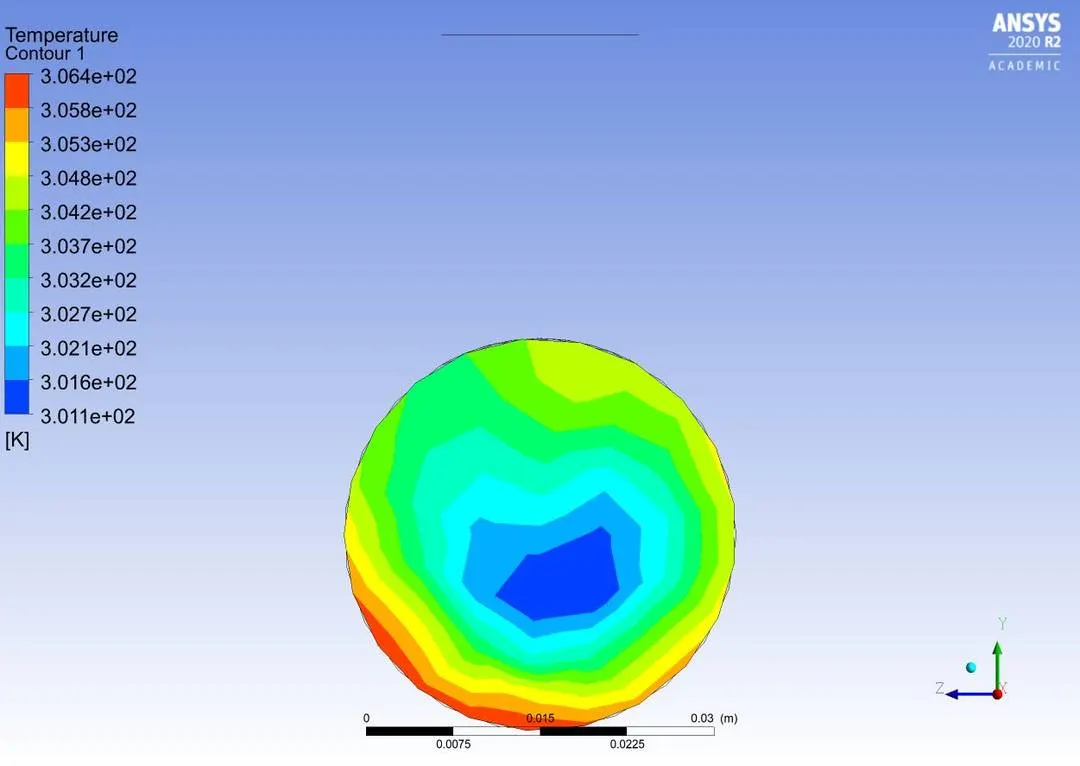
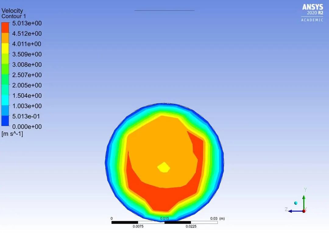
CASE 2: momentum ratio - 2; k-omega solver; mesh size: 5mm; size: short

CASE 3: momentum ratio - 2; k-omega solver; mesh size: 1.5mm; size: short

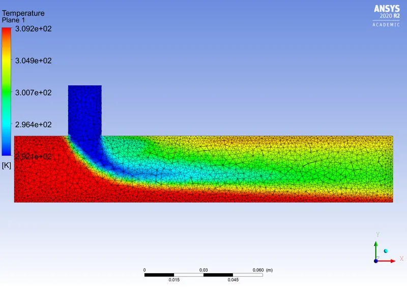
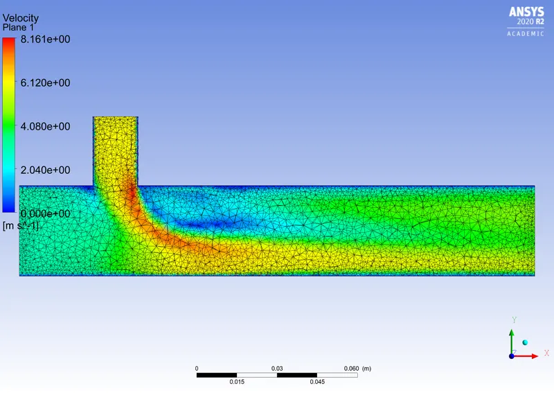
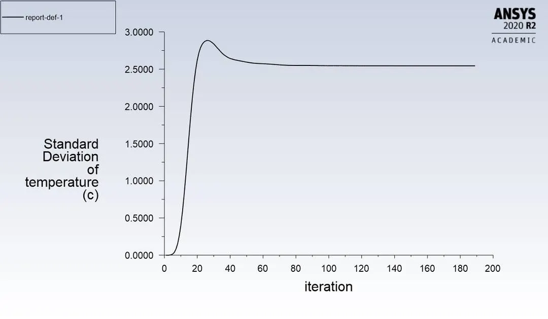
CASE 4: momentum ratio - 2; k-omega solver; mesh size: 3mm; size: short

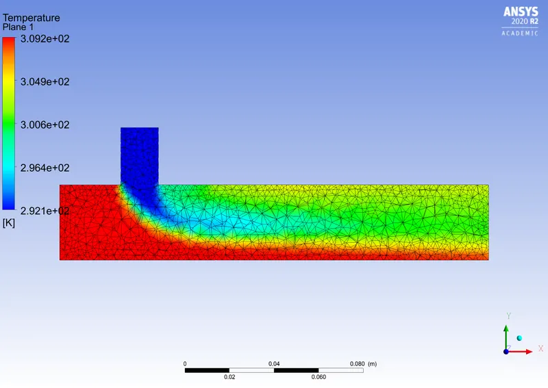
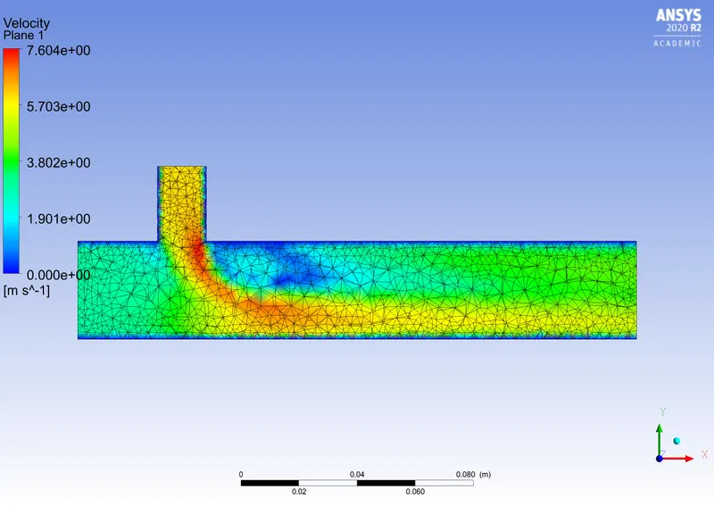
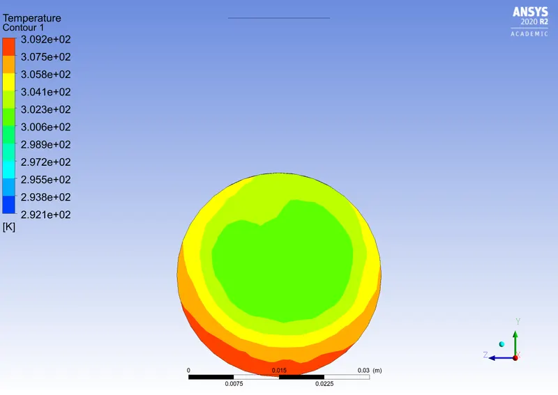
CASE 5: momentum ratio - 4; k-omega solver; mesh size: 5mm; size: short

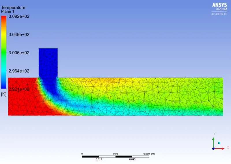
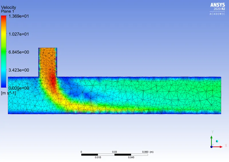
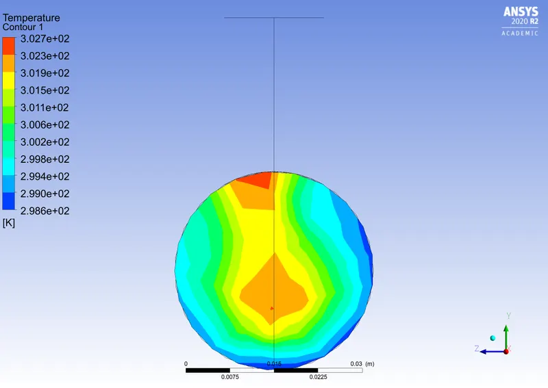
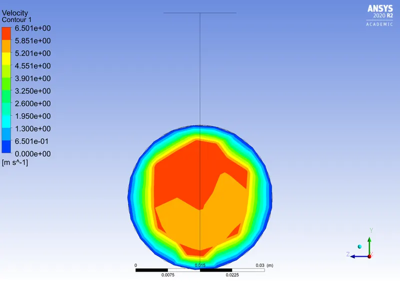
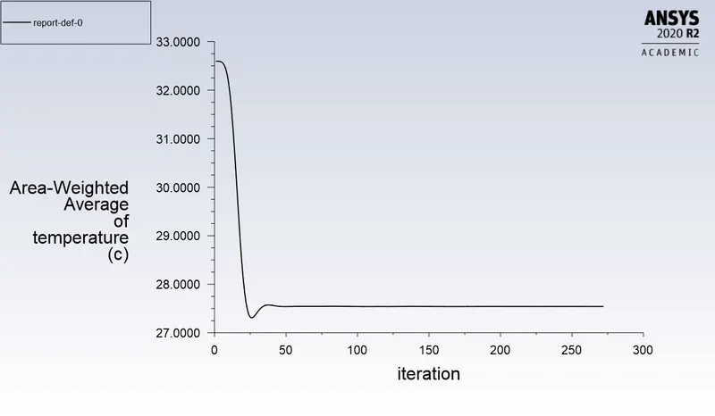
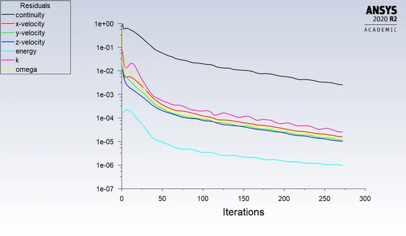
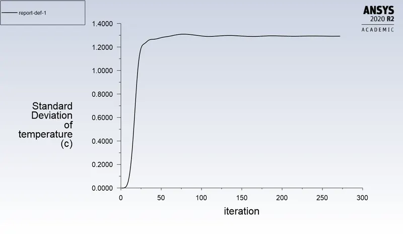
CASE 6: momentum ratio - 2; k-omega solver; mesh size: 5mm; size: long

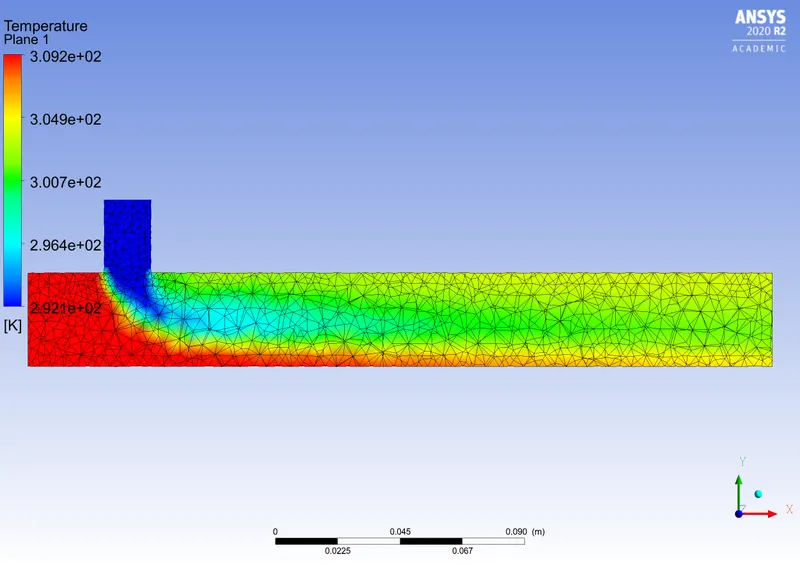
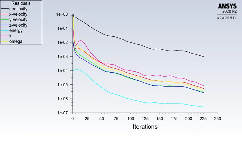
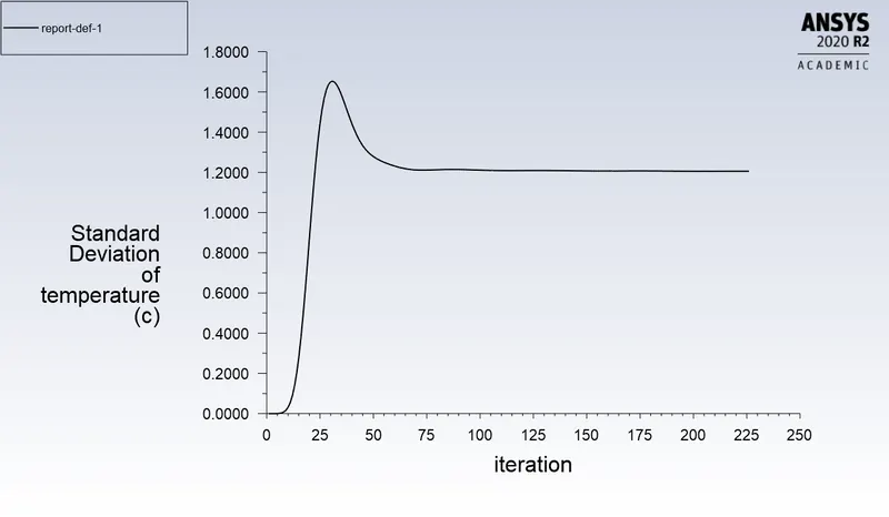
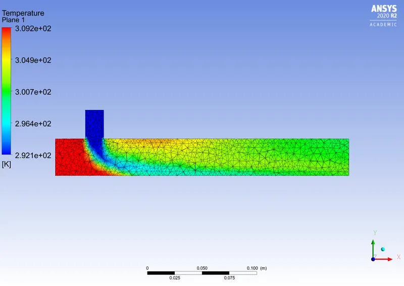
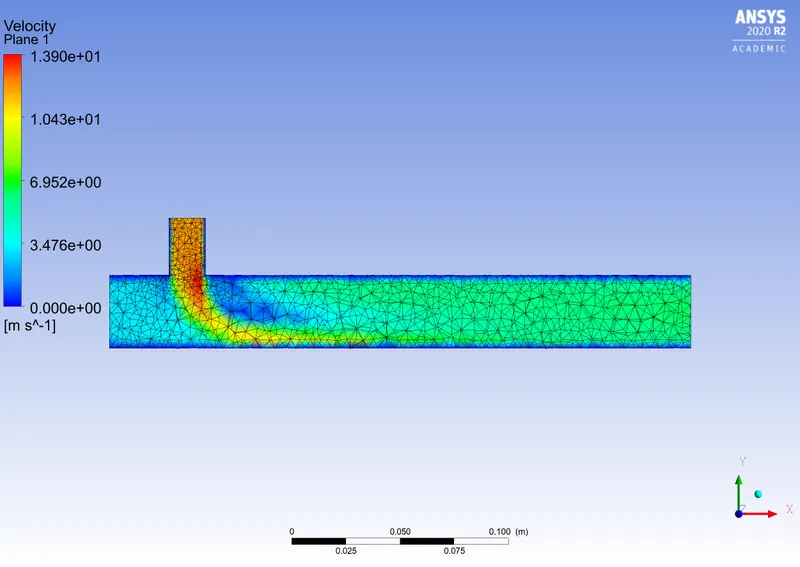
CASE 6: momentum ratio - 4; k-omega solver; mesh size: 5mm; size: long

CONCLUSIONS:

• We use k-omega SSt as it is a hybrid between k-omega and k-episilon, the sst solver gives us k-episilon type solution away from the wall and k-omega type solution near the wall
• By changing the mesh size between 1.5mm, 3mm, 5mm. we can see that the solution is not mesh size dependent.
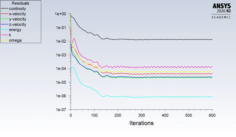
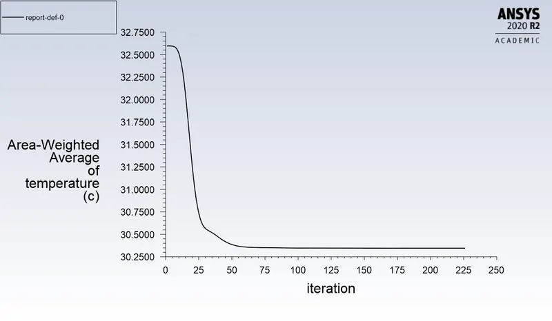
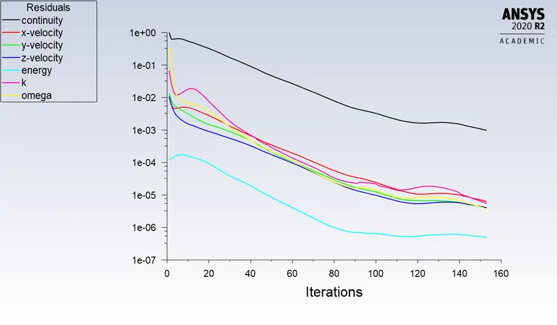
• The value of the residuals are continuously decreasing and the solutions converge.
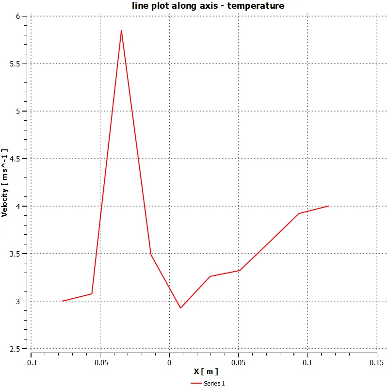
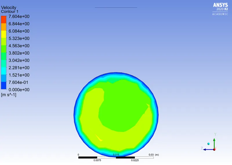
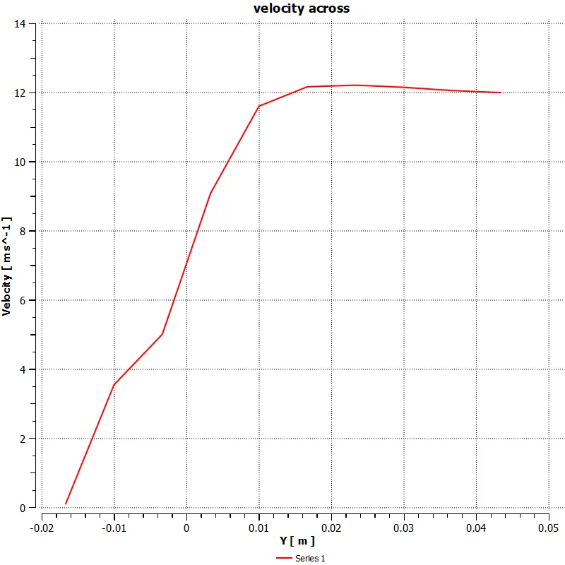
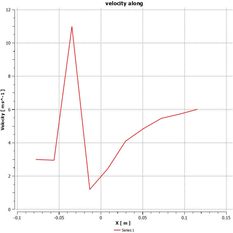
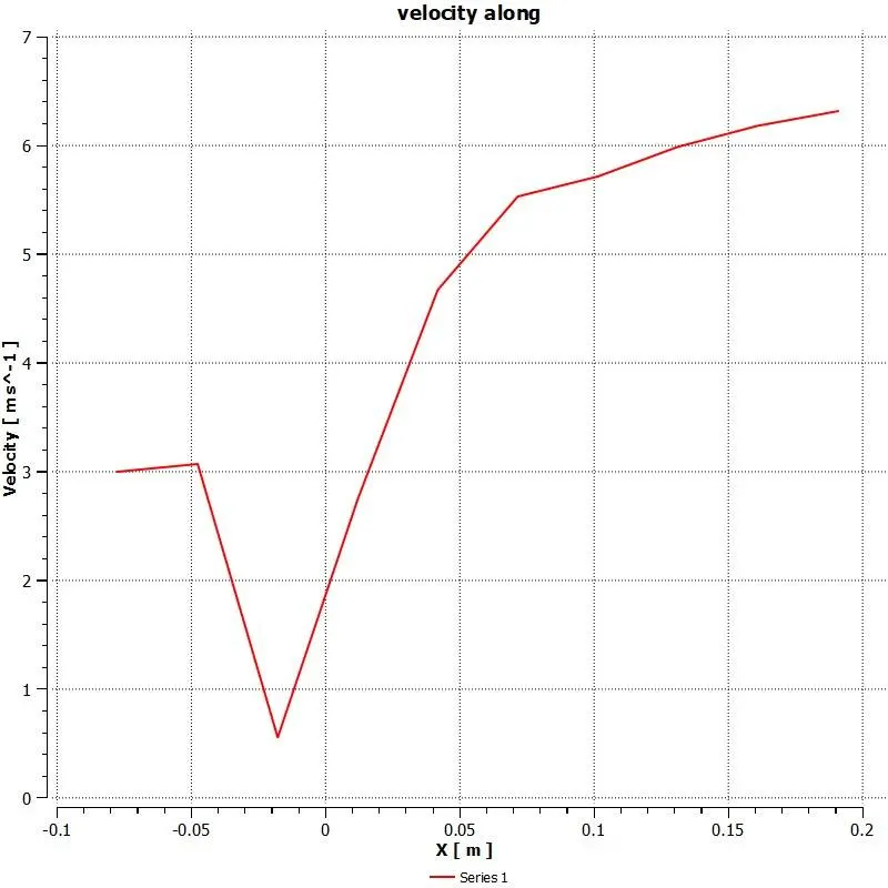
• From all the velocity contours we can see that the velocity at the walls are zero, and greater towards the middle. this follows the physics of the problem.
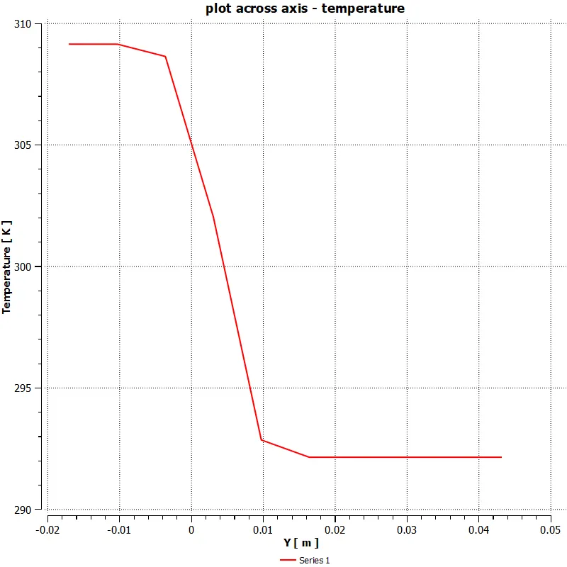
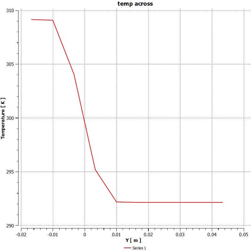
• From the temperature contours we can see thart the hot air from the inlet-x is stil present at the bottom of the contour.
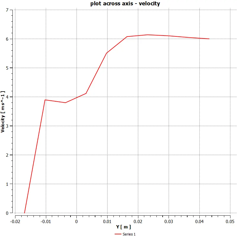
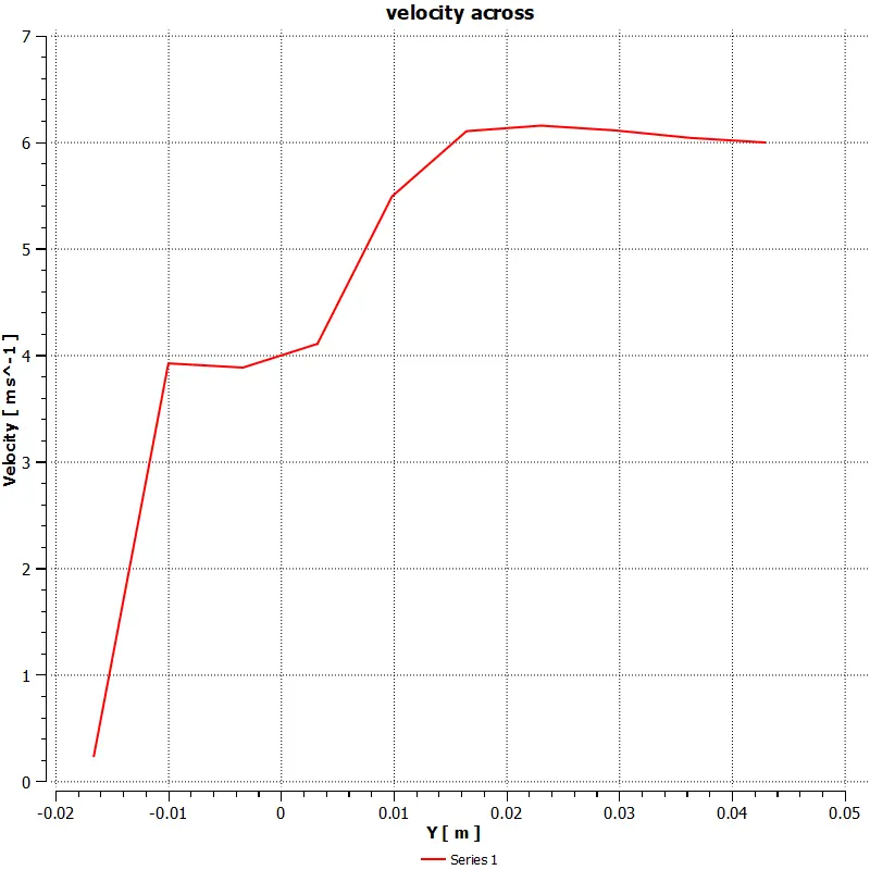
• From the velocity across plot we can see that the velocity at the begining is zero, this is in accordance with the physics, which states that the velocity at the boundary is 0
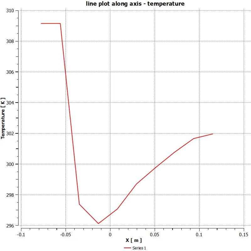
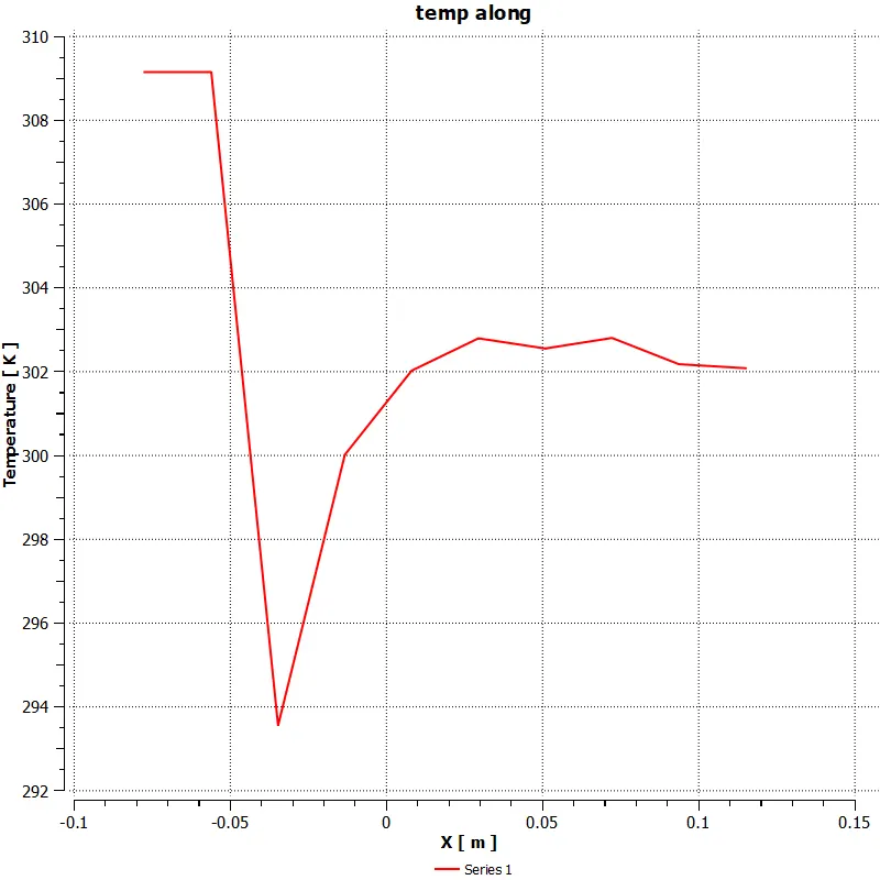
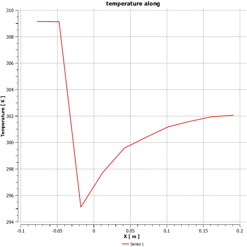
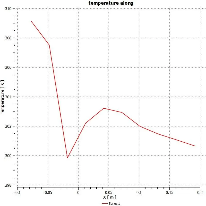
• From the temperature along graph we can see that the temperature steadily decreases as the cold air from inlet-y enters the stream, and then increases as mixing takes place.
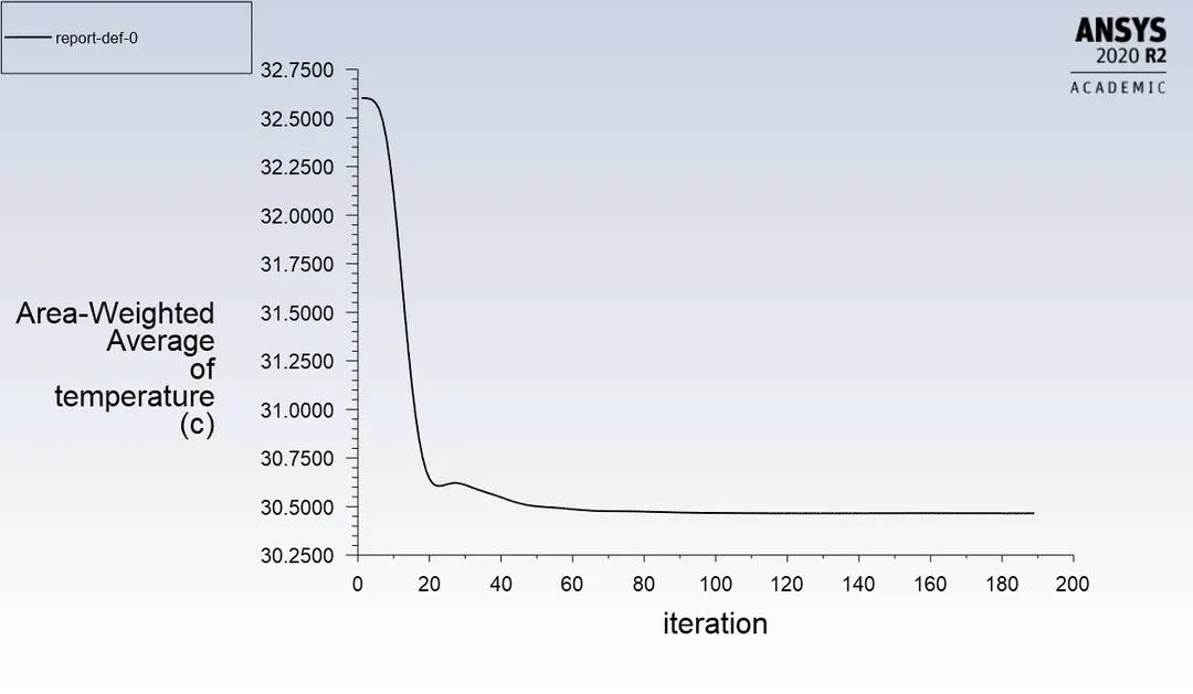
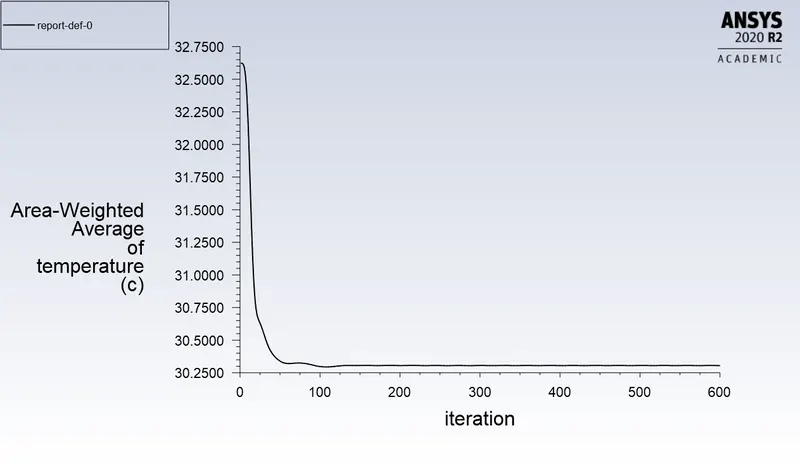
• From the area weighthed average of the temperature taken at the outlet we can see that the predicted temperature is slightly above the predicted temperature, though the k-omega solver provides a slightly more accurate solution.
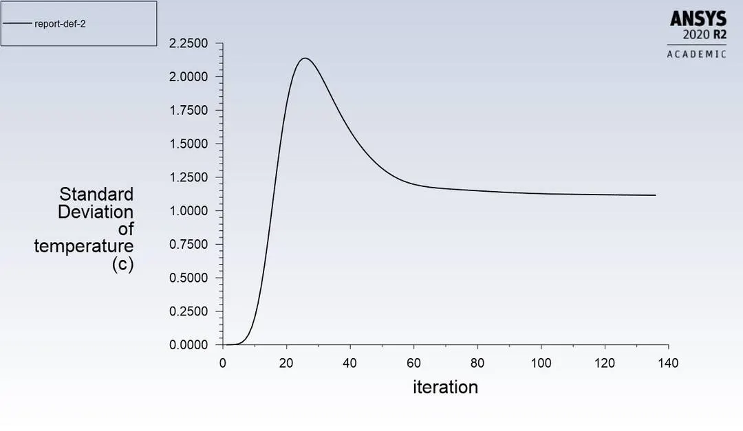
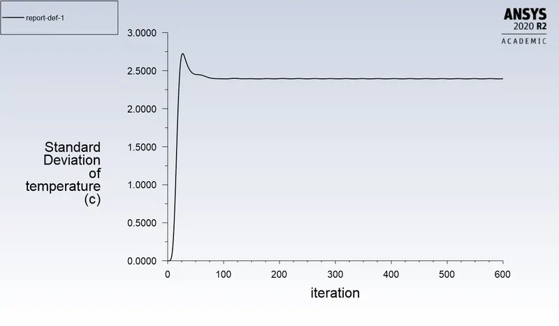
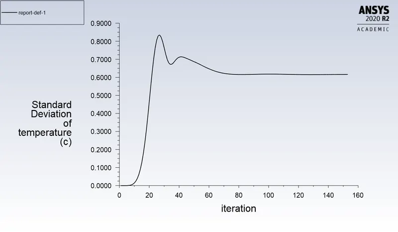
• We can see from the standard deviation graph and the contours that the mixing efficiency of the long tee is better than that of the short tee.
• We can see that the area weighted average temperature shows only a significant change when the the momentum ratio is changed.
• when we change the size of the mesh from 5 mm to 1.5mm and 3mm we can see that the values do not change that much, thus we can say that teh grid independence test was sucessful