Week 4 - Genetic Algorithm

AIM :

To understand the genetic algorithm and successfully apply it to a function to calculate the maxima.

OBJECTIVE:

• Write a code in MATLAB to optimise the stalagmite function and find the global maxima of the function.
• Plot graphs for all 3 studies and for F maximum vs no. of iterations.

FORMULAE USED:

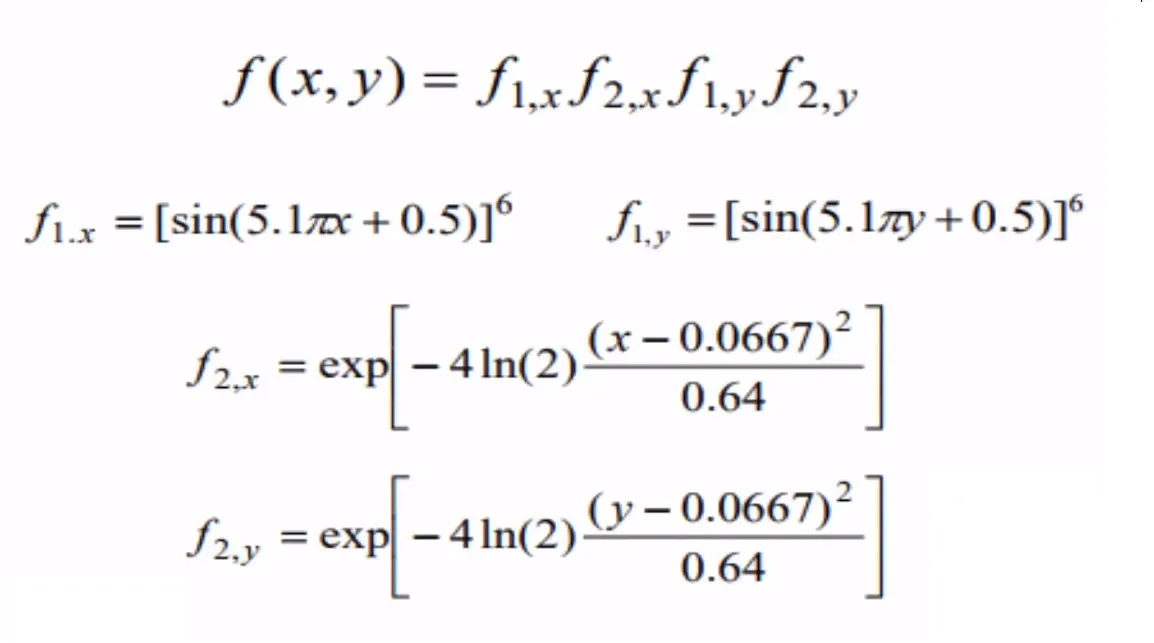
the formulae for the stalagmite function is mentioned below

THEORY:

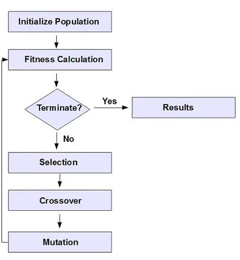
The genetic algorithm solver in MATLAB makes use of Darwin's theory of natural selection to perform optimization. It is an extremely powerful solver that can be used in multiple ways, passing multiple conditions. The GA returns the minima, thus to obtain the maxima or other statistics the function passed must be appropriately modified

The GA is frequently used to find optimal or near-optimal solutions to difficult problems which otherwise would take a lifetime to solve. It is frequently used to solve optimization problems, in research, and in machine learning.

CODE:

major functions used in code

• Gentic algorithm:[position,fval(i)]=ga(@stalagmite,2); - calling the ga solver by sending the stalagmite function(also the number of variables '2') and outputting the position in the matrix and the minima value at the point.( note: the GA solver is cxalled in multiple way throughout the code)
• subplot()- used to plot multiple graphs in 1 figure.
• shading interp - to make the plot easier to visualise.
• surfc() - to visualise the plot
• options=optimoptions('ga'); returns options with the named parameters altered with the specified values
• options=optimoptions(options,'PopulationSize',num_cases_1) to specify the population size parameter with the value of num_cases_1

%stalagmite function using ga
clear all
close all
clc

%defining search space
x=linspace(0,0.6,150);
y=linspace(0,0.6,150);
num_cases =50; %GA without mentioning population does 50 iterations 

%defining 2dimentional mesh 
[xx yy]=meshgrid(x,y );

%evaluating stalagmite
for i=1:length(xx)
    for j=1:length(yy)
        input_vector(1)=xx(i,j);
        input_vector(2)=yy(i,j);
        f(i,j)=stalagmite(input_vector); % calling the stalagmite function.
    end
end

%to check the position of outputs of the ga function
for i=1:num_cases
    [position,fval(i)]=ga(@stalagmite,2); % calling the ga without any conditions
    x_output1(i)= position(1); %storing the x coordinate of the output
    y_output1(i)= position(2); %storing the y coordinate of the output
end

figure(1)
subplot(2,1,1); % to plot more than one graph in the figure ,1st graph
surfc(xx,yy,f) % to visualise the plot
hold on
xlabel('xaxis');
ylabel('ylabel');
shading interp ; % to make it easier to visualise 
plot3(x_output1,y_output1,fval,'marker','*','markersize',5,'markerfacecolor','r'); % to provide the markers of the ga iterations.
title('unbounded inputs');
subplot(2,1,2); % to plot more than one graph in the figure ,2nd graph
plot(fval);
xlabel('iterations');
ylabel('function minimum');


% study 2 with boundary conditions
%to check the position of outputs of the ga function
for i=1:num_cases
    [position,fval(i)]=ga(@stalagmite,2,[],[],[],[],[0,0],[1,1]); % applying boundry conditions to the ga function
    x_output1(i)= position(1);  %storing the x coordinate of the output
    y_output1(i)= position(2);  %storing the y coordinate of the output
end


figure(2)
subplot(2,1,1); % to plot more than one graph in the figure ,1st graph
surfc(xx,yy,f) % to visualise the plot
hold on
xlabel('xaxis');
ylabel('ylabel');
shading interp ; % to make it easier to visualise 
plot3(x_output1,y_output1,fval,'marker','*','markersize',5,'markerfacecolor','r'); % to provide the markers of the ga iterations.
title('bounded inputs');
subplot(2,1,2); % to plot more than one graph in the figure ,2ndgraph
plot(fval);
xlabel('iterations');
ylabel('function minimum');

num_cases_1= 170;
%study 3 with increasing the iterations
options=optimoptions('ga');
options=optimoptions(options,'PopulationSize',num_cases_1); % to increase the number of iterations

%to check the position of outputs of the ga function
for i=1:num_cases_1
    [position,fval(i)]=ga(@stalagmite,2,[],[],[],[],[0,0],[1,1],[],[],options); % applying boundry conditions to the ga function with increase in iterations.
    x_output1(i)= position(1);  %storing the x coordinate of the output
    y_output1(i)= position(2);  %storing the y coordinate of the output
end

figure(3)
subplot(2,1,1); % to plot more than one graph in the figure ,1st graph
surfc(xx,yy,f) % to visualise the plot
hold on
xlabel('xaxis');
ylabel('ylabel');
shading interp ; % to make it easier to visualise 
plot3(x_output1,y_output1,fval,'marker','*','markersize',5,'markerfacecolor','r'); % to provide the markers of the ga iterations.
title('bounded inputs with increased population');
subplot(2,1,2); % to plot more than one graph in the figure, 2nd graph
plot(fval);
xlabel('iterations');
ylabel('function minimum');

The stalagmite function is shown below.the whole function is multiplied by -1 to return the maxima as the ga solver returns minima, thus by multiplying the entire function by -1 we are able to find the maxima using the GA solver

%function - stalagmite

function [g]= stalagmite(input_v)
term_1 = (sin((5.1*pi*input_v(1))+0.5))^6;
term_2 = (sin((5.1*pi*input_v(2))+0.5))^6;
term_3 = exp(-4*log(2)*(((input_v(1)-0.0667)^2)/0.64));
term_4 = exp(-4*log(2)*(((input_v(2)-0.0667)^2)/0.64));
g= -1*term_1*term_2*term_3*term_4; % entire function multipled by -1 to find maxima using GA solver
end

OUTPUT:

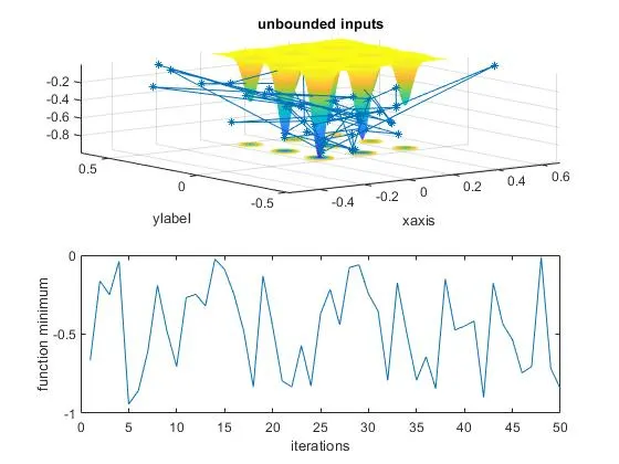
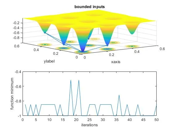
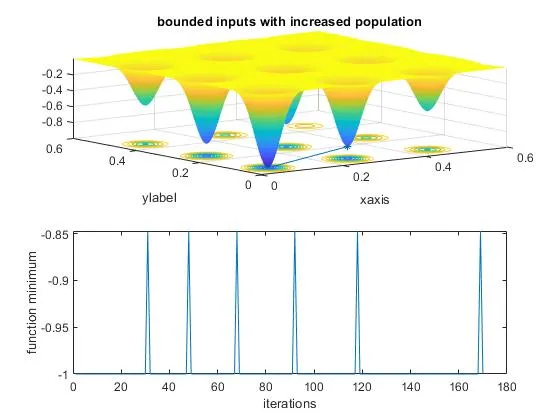
The output of the code is as shown below.

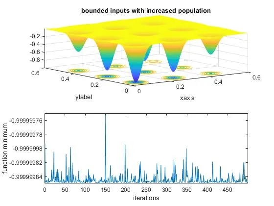
When the number of iterations is increased to 500 this is the graph that is displayed

CONCLUSIONS:

From the output graphs we can understand:

• In the first output graph we can see that when the solver is unbounded the GA go outside the range of the stalagmite function and the GA solver does not return consistant values
• In the second output graph we can see that when the conditions are bounded the GA solver ends up working much better, though the solver returns various local minima
• In the first 2 graphs we can see that the solver does not return accurate values of function minimum, these values also change drastically
• In the 3rd graph we can see that as we increase the number of iteration to 170, the solver startes to become more accurate and consistantly returns the function minimum as-1 though local minima are also outputted.
• In the final graph we can see that as we increase the number of iterations drastically to 500 that the solver is much more accurate and the change in the value of function minimum varies only on the order of 0.0000001 this is a drastic improvement and the best solution so far.
• We can also see that as the number of iterations increase the time taken for the code to be executed also increases quite substantially.