Rayleigh Taylor Instability Challenge

AIM:

To understand the Rayleigh-Taylor Instability

OBJECTIVE:

1. What are some practical CFD models that have been based on the mathematical analysis of Rayleigh Taylor waves? In your own words, explain how these mathematical models have been adapted for CFD calculations.
2. Perform the Rayleigh Taylor instability simulation for 2 different mesh sizes with the base mesh being 0.5 mm. Compare the results by showing the animations( Attach them from your google drive). Observe the differences in the animation and explain the effect of mesh size on simulation. Also, explain why a steady-state approach might not be suitable for these types of simulation.[ Choose Air and Water for this simulation]
3. Run one more simulation with water and user-defined material(density = 400 kg/m³, viscosity = 0.001 kg/m-s) for refined mesh.
4. Define the Atwood Number. Find out the Atwood number for both the cases and explain how the variation in Atwood number in the above two cases affects the behavior of the instability.

THEORY:

ATWOOD number:

The Atwood number (A) is a dimensionless number in fluid dynamics used in the study of hydrodynamic instabilities in density stratified flows. It is a dimensionless density ratio defined as

where

= density of heavier fluid

= density of lighter fluid

Atwood number is an important parameter in the study of Rayleigh–Taylor instability and Richtmyer–Meshkov instability. In Rayleigh–Taylor instability, the penetration distance of heavy fluid bubbles into the light fluid is a function of acceleration time scale.

Atwood number for the air-water combination= 0.997

Atwood number for the userdefined -water combination(density = 400 kg/m³, viscosity = 0.001 kg/m-s) = 0.428

The value of the atwood number affects the nature of the instability, when atwood number is close to 0 the instability takes the form of symmetric fingers of fluid, when atwood number is closer to 1 the heavier fluid takes the form of large bubble like plumes.

Rayleigh-Taylor Instability:

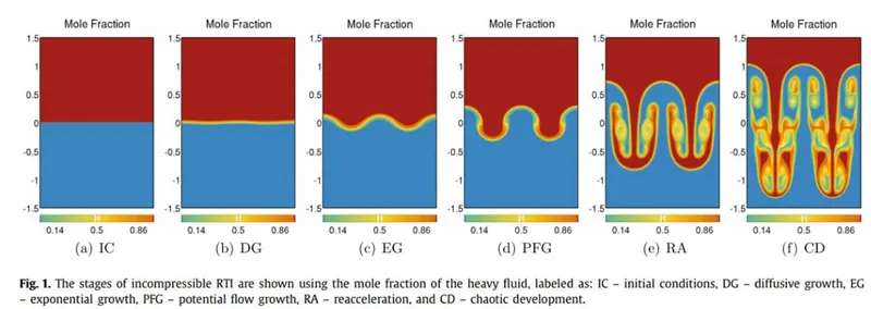
Rayleigh-Taylor instability (RTI) is the interpenetration of materials that occurs whenever a light fluid pushes on a heavy fluid (Rayleigh 1883, Taylor 1950). It is a dynamic process whereby the two fluids seek to reduce their combined potential energy. The ensuing turbulence and mixing has far-reaching consequences in many natural and man-made flows, ranging from supernovae to inertial confinement fusion (ICF) capsules.

The fact that RTI grows up from small scales presents a challenge to numerical computations employing the large-eddy simulation (LES) methodology. Subgrid-scale (SGS) models that assume a turbulent cascade of energy from large to small scales do not apply at early times when kinetic energy is generated at perturbation length-scales far below the grid scale. RTI also presents a challenge to computations employing the Reynolds-averaged Navier-Stokes (RANS) method since "turbulent diffusion" models

Transient state over steady state:

In the Rayleigh- Taylor Instability, due to a sudden collapse in the layer between the denser and lighter fluid spike generation takes place which is obviously time dependent,hence using a steady state solver will not work as we are interested in the flow parameters with respect to time.

CFD models based on analysis of Rayleigh-Taylor waves

1. Richtmyer-Meshkov Instability(RMI): occurs when two fluids of different density are impulsively accelerated. Normally this is by the passage of a shock wave. The development of the instability begins with small amplitude perturbations which initially grow linearly with time. This is followed by a nonlinear regime with bubbles appearing in the case of a light fluid penetrating a heavy fluid, and with spikes appearing in the case of a heavy fluid penetrating a light fluid. A chaotic regime eventually is reached and the two fluids mix. This instability can be considered the impulsive-acceleration limit of the Rayleigh–Taylor instability.
2. Kelvin-helmholtz Instability:typically occurs when there is velocity shear in a single continuous fluid, or additionally where there is a velocity difference across the interface between two fluids. A common example is seen with wind blowing over water, the instability constant is able to manifest itself through waves on a water surface. The Kelvin-Helmholtz instability is not only restricted to a water surface as clouds, but is evident through other natural phenomena as the ocean, Saturn's bands, etc.
3. Plateau-Rayleigh Instability: explains why and how a falling stream of fluid breaks up into smaller packets with the same volume but less surface area. It is related to the Rayleigh–Taylor instability and is part of a greater branch of fluid dynamics concerned with fluid thread breakup.The driving force of the Plateau–Rayleigh instability is that liquids, by virtue of their surface tensions, tend to minimize their surface area. A considerable amount of work has been done recently on the final pinching profile by attacking it with self-similar solutions.

CASE SETUP

Geometry:

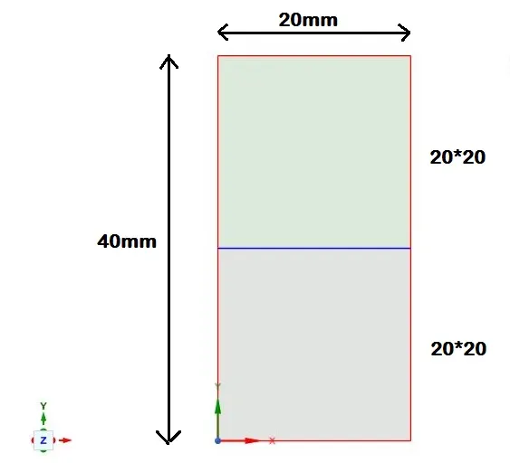
1) Open spaceclaim -> draw the geometry (2 20 mm squares stacked on each other) using 'rectangle';
2) Use the pull tool to make the rectangle into a plane.
3) Share topology to get a shared surface between the 2 squares.

Meshing:

1. Open meshing interface and click generate mesh (this will create base mesh).
2. Name the surfaces.
3. Refine the mesh by changing mesh size, run two cases 0.5mm and 0.25 mm (mesh images are shown below in results for the coarse and refined mesh)

Fluent:

1. Launch fluent -> transient simulation (because we require a time accurate solution); gravity enabled(as -9.81 in y direction to simulate gravity);pressure based (as compressibility effects are not in the picture); absolute velocity.
2. Select a laminar flow simulation as that is the problem definition.
3. Enable the multiphase model -> select the volume of fluid method ; 2eulerian faces ; implicit formulation (since there are 2 materials of different phases, we also want an implicit simulation to be done).
4. Materials -> fluent database -> copy 'water - liquid' - in phases list the phases accordingly (we are doing this to define the materials in the 2 phases of the problem).
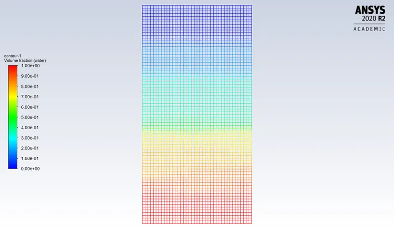
5. Solution -> initialise (standard) -> patch -> phase : water -> volume fraction -> 1 for the water region (above) 0 for the air region. the patch must be created before everysimulation. (we do patching to initialise the volume fraction as in this case there is an extra equation that needs to be solved).
6. Create the contour plot of the geometry this will help in seeing if the patching was done correctly, and provide the base for the animation.
7. Create animation to visualise the flow.
8. Enter time step size =0.005; no of time steps =700;

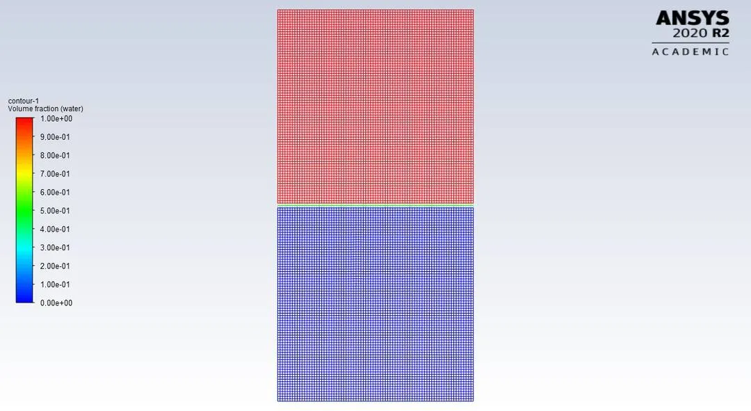
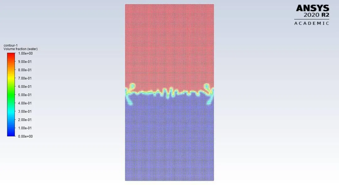
from the above image we can see that the patching has been done accurately

SIMULATIONS RUN:

1. Air -water, coarse mesh (0.5mm).
2. Air -water, refined mesh (0.25mm).
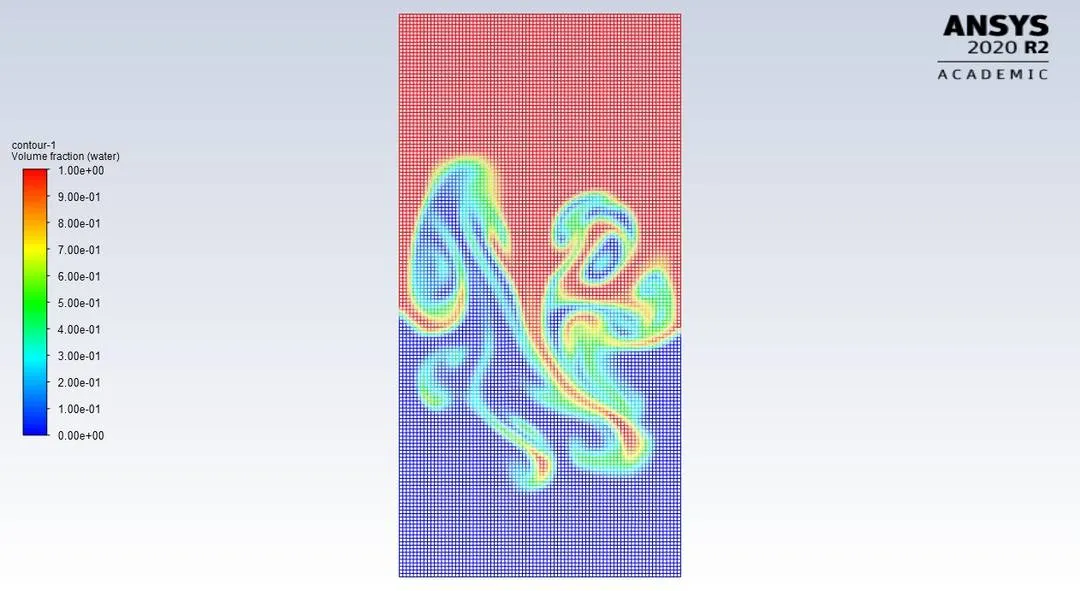
3. User defined material -water, refined mesh (0.25mm)

RESULTS:

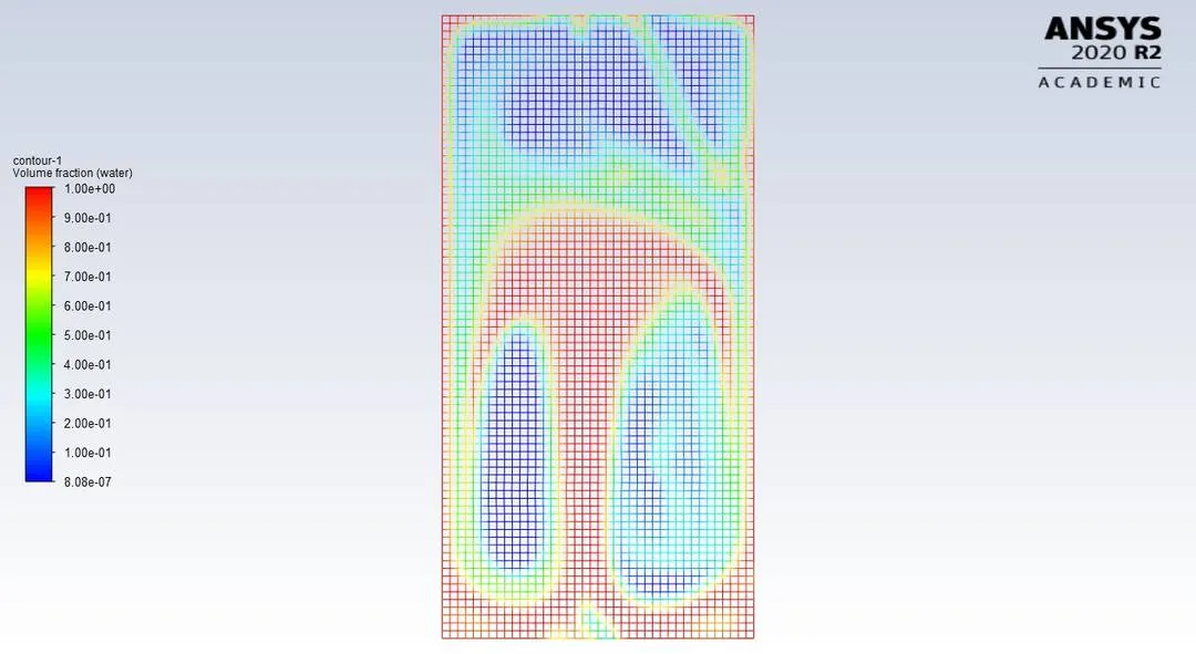
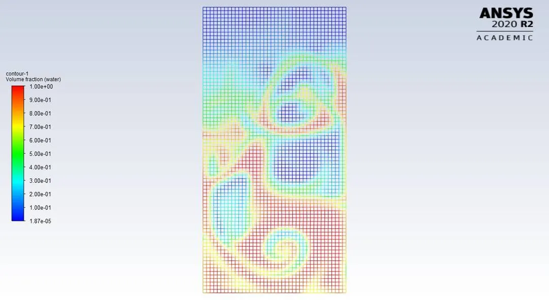
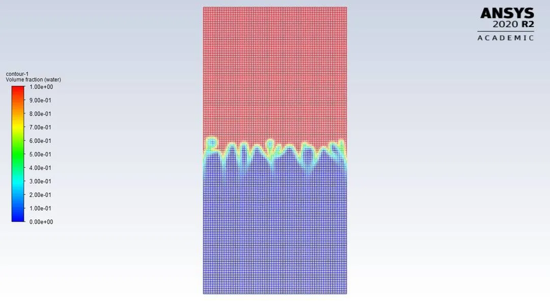
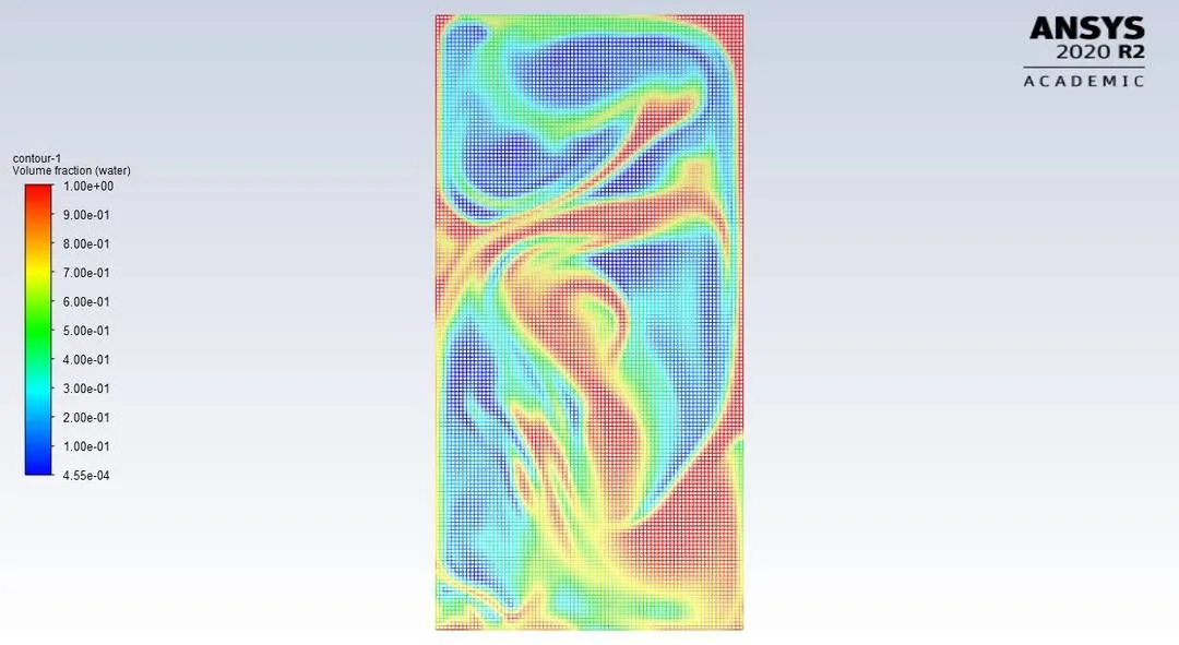
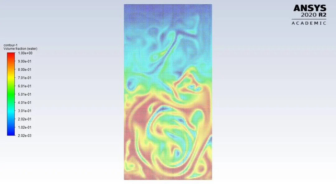
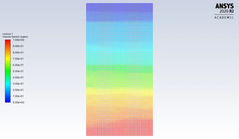
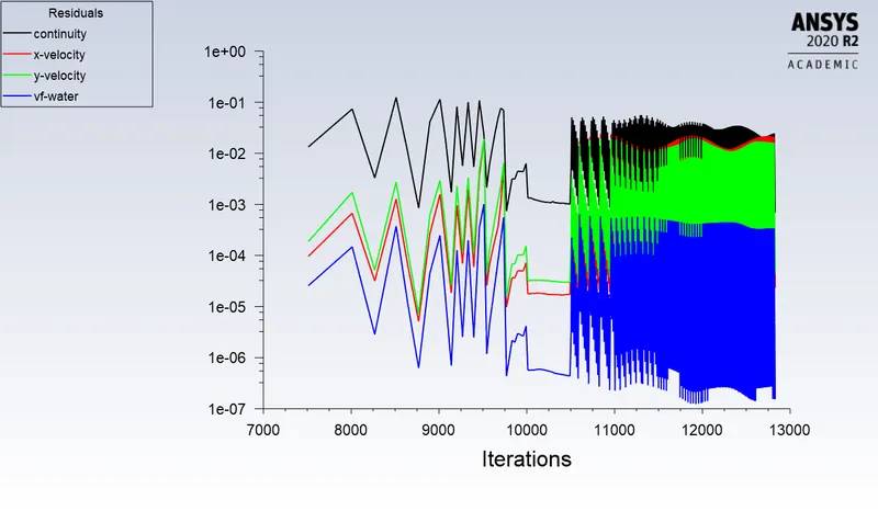
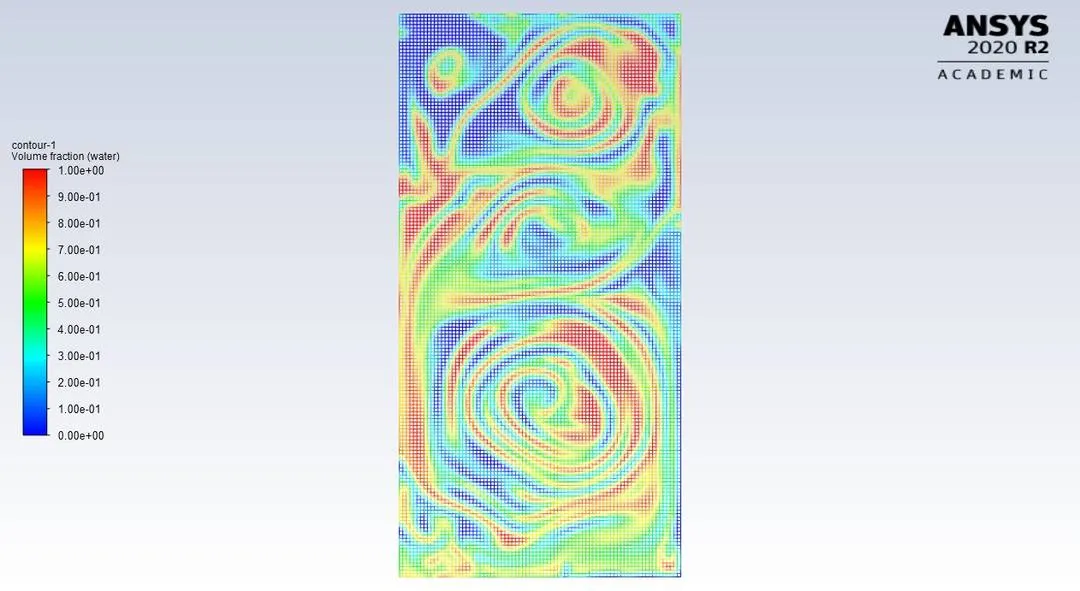
Given below are the images of the 3 simulations at 4 different time steps.

case1:Air -water, coarse mesh (0.5mm).

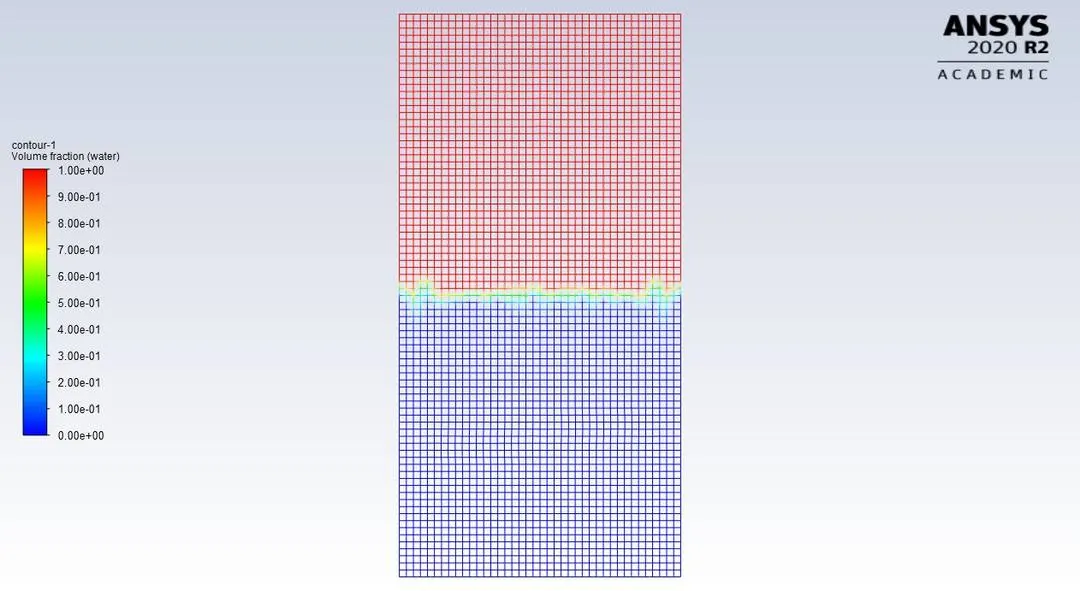
Simulation animation: CASE1 animation

case 2: Air -water, refined mesh (0.25mm).

Simulation animation: CASE2 animation

case 3: User defined material -water, refined mesh (0.25mm)

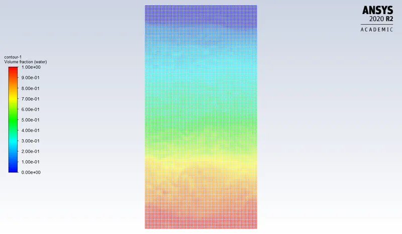
Simulation animation: case3 animation

CONCLUSIONS:

• We can see that as we increase the mesh size the diffusion increases and the capturing of the instability is compromised.
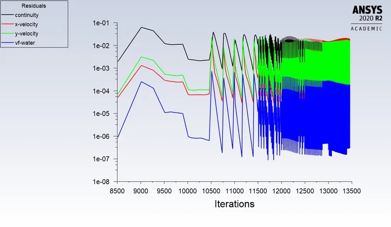
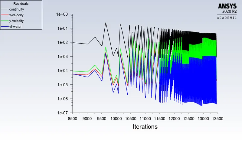
• Incorrect or large time step causes 'floating point exception' error, this results in a sudden increase in residuals during run time.
• coarse mesh attains steady state faster.
• Finer mesh is better at capturing the physics but will take more time steps in reaching the steady state, thus will also take more computational time.
• we are able to see bubbles and spikes in the simulation.
• The value of the atwood number affects the nature of the instability, when atwood number is close to 0 the instability takes the form of symmetric fingers of fluid, when atwood number is closer to 1 the heavier fluid takes the form of large bubble like plumes.
• At the end of the simulation, though the two phases are seperated from each other, there is a certain amount of diffusion that takes place.