Conjugate Heat Transfer Analysis on a graphics card. (ANSYS FLUENT)
AIM :
To perform CHT analysis on a graphics card
OBJECTIVE:
- Run the simulation by varying the velocity from 1m/sec to 5m/sec for at least 3 velocities and discuss the results.
- Find out the maximum temperature and heat transfer coefficient attained by the processor.
- Prove that the simulation has achieved convergence with appropriate images and plots.
- Identify potential hotspots on the model.
THEORY:
CHT Analysis:
CHT stands for Conjugate Heat Transfer,
Conjugate heat transfer corresponds with the combination of heat transfer in solids and heat transfer in fluids. In solids, conduction often dominates whereas in fluids, convection usually dominates. Conjugate heat transfer is observed in many situations. For example,
Heat Transfer by Solids and Fluids
Heat Transfer in a Solid
In most cases, heat transfer in solids, if only due to conduction, is described by Fourier’s law defining the conductive heat flux, q, proportional to the temperature gradient:  .
.
For a time-dependent problem, the temperature field in an immobile solid verifies the following form of the heat equation:

Heat Transfer in a Fluid
Due to the fluid motion, three contributions to the heat equation are included:
- The transport of fluid implies energy transport too, which appears in the heat equation as the convective contribution. Depending on the thermal properties on the fluid and on the flow regime, either the convective or the conductive heat transfer can dominate.
- The viscous effects of the fluid flow produce fluid heating. This term is often neglected, nevertheless, its contribution is noticeable for fast flow in viscous fluids.
- As soon as a fluid density is temperature-dependent, a pressure work term contributes to the heat equation. This accounts for the well-known effect that, for example, compressing air produces heat.
Accounting for these contributions, in addition to conduction, results in the following transient heat equation for the temperature field in a fluid:

- Open space claim, import the geometry
- check for interference.
- enable share topology, and click 'tick';
- add the second enclosure for refinement.
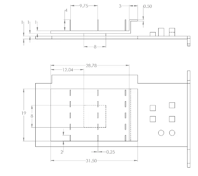
- Open the meshing interface.
- Name the inlet, outlet and the outer walls (wall-symmetry)
- For the coarse mesh, right click(r.c) on mesh and click generate mesh.
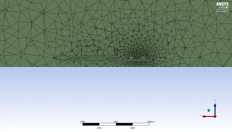
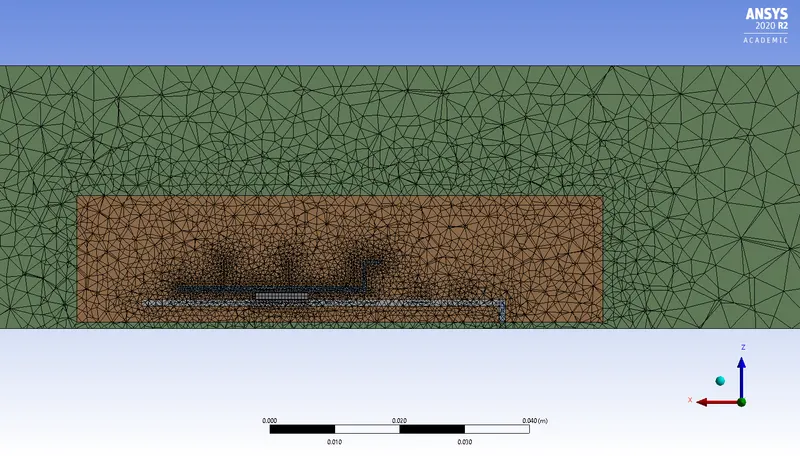
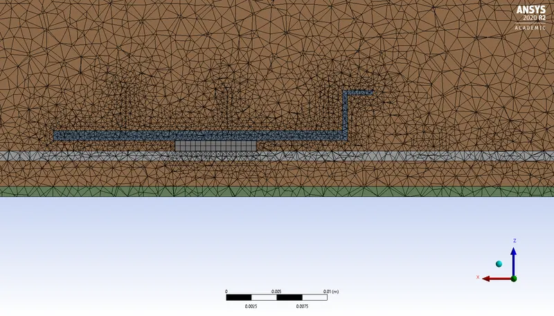
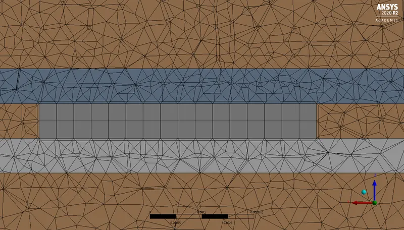
- From the above coarse mesh we can see that it does not properly capture the features properly, thus we need to refine the mesh in areas of interest. For the refined mesh, r.c on mesh -> insert sizing -> select the body and give the mesh size.
processor -0.5mm (we require the best possible mesh to capture the features as this is an area of great importance )
fins- 0.5mm (we require the best possible mesh to capture the features as this is an area of great importance )
pcb- 1mm (the mesh is slightly less refined as the material of the pcb does not transfer much hear thus we can increase the mesh size here )
inner enclosure - 5mm(by making the inner enclosure finer we are able to better capture the flow in this region)
outer enclosure - 10mm (standard mesh size) - Ensure mesh conformity.
below is the image for coarse mesh.
- Open ansys fluent -> physics-> pressure based, absolute ,steady state, k-epsilon solver(realisable).
- Physics -> materials -> set materials -> set up boundary conditions for components.
inlet velocity :
case 1: 5m/s
case 2 : 3m/s
case 3: 1m/s - In materials, add different material
fins-> aluminium (available in fluent database)
density : 2719 kg/m^3
heat capacity: 871 J/KgK
thermal conductivity : 202.4 W/mK
processor -> silicon
density :2000 kg/m^3
heat capacity: 710 J/KgK
thermal conductivity : 150 W/mK
PCB-> FR4
density : 1890 kg/m^3
heat capacity: 950 J/KgK
thermal conductivity : 0.29 W/mK
fluid-> air (available in fluent database)
density : 1.225 kg/m^3
heat capacity: 1006.43 J/KgK
thermal conductivity : 0.0242 W/mK - In cell zones make sure to specify the sections properly as either solid or fluid.
- In cell zones -> click source terms (only for processor)-> heat generation =2.34 e7 W/M^3 (calculated from real world examples)
- Solution -> initialise -> enter no of iterations
- Create the required plots
- Hit calculate to run the simulation
RESULTS:
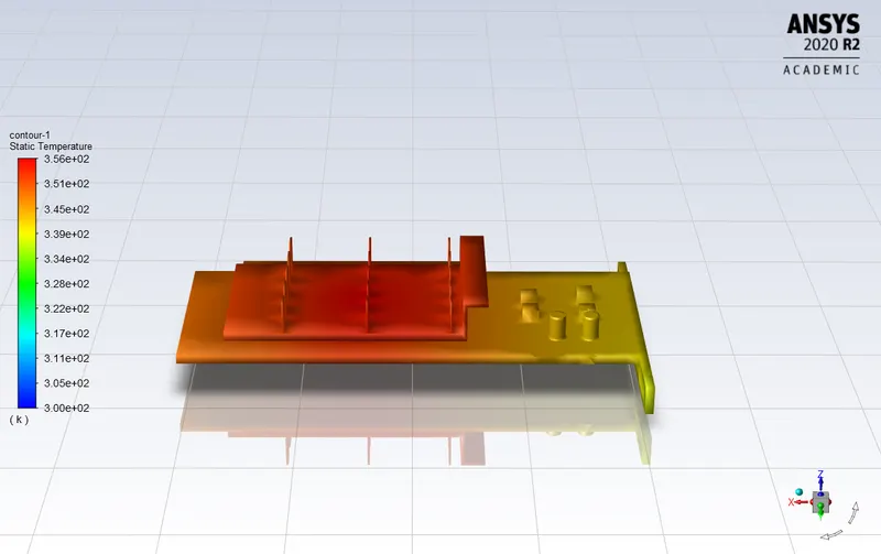
case 0: Coarse mesh (all materials are aluminium)
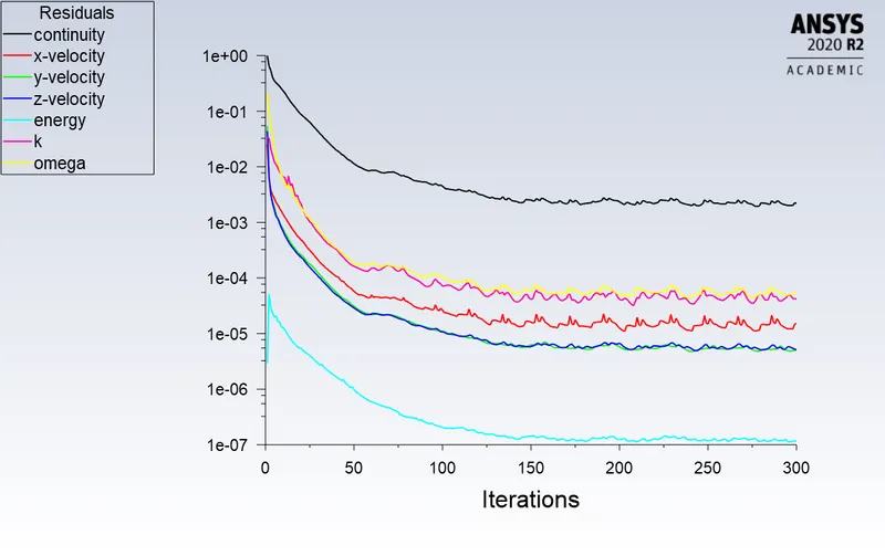
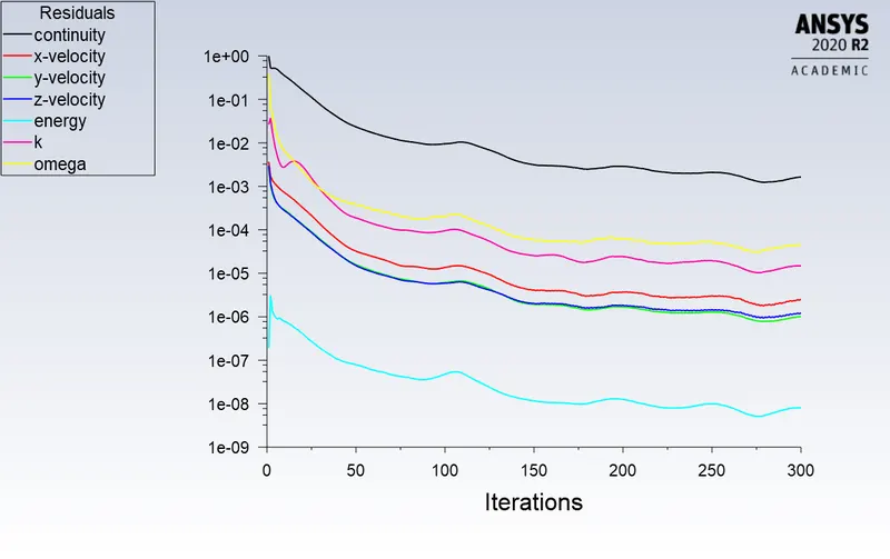
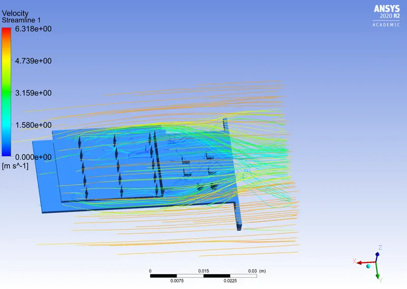
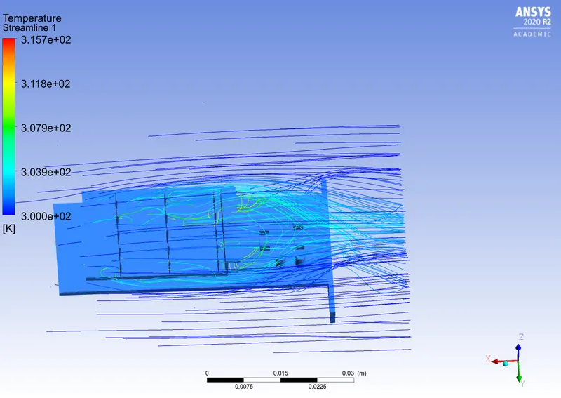
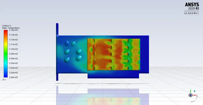
CASE 1: Refined mesh, inlet velocity 5 m/s (materials have been defined as above)
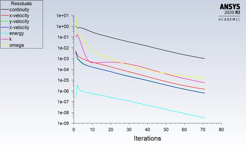
below is the graph of the residuals, we can see that the solution has converged (convergence criteria has been specified as the default values )
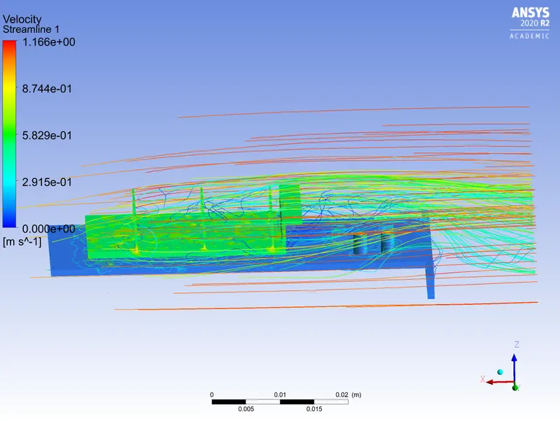
velocity streamlines
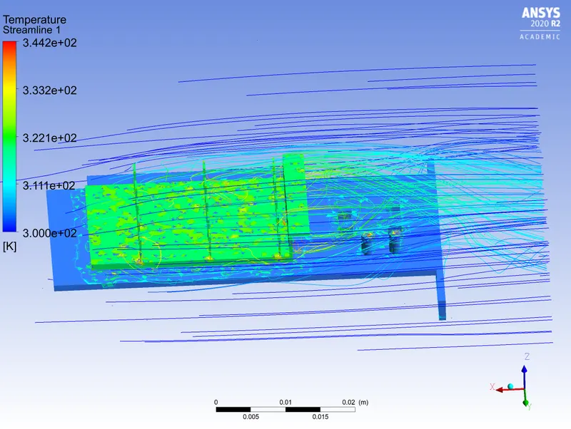
Temperature Streamlines
Temperature contours
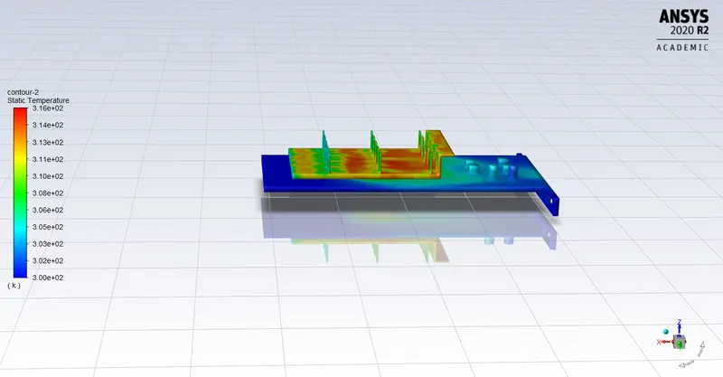
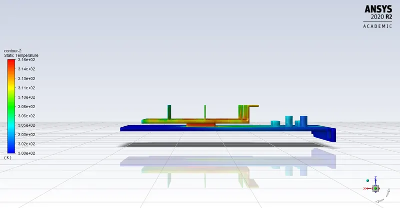
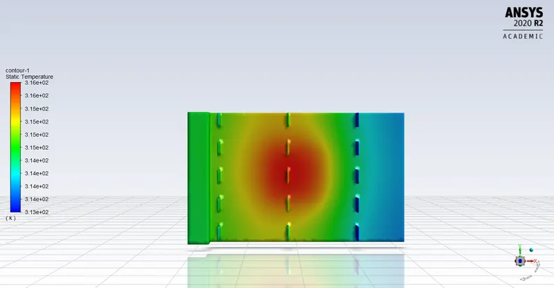
Local temperature contour for the fin
temperature plane contour 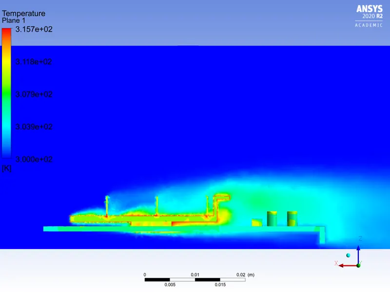
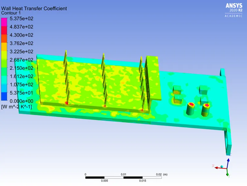
wall heat transfer coefficient
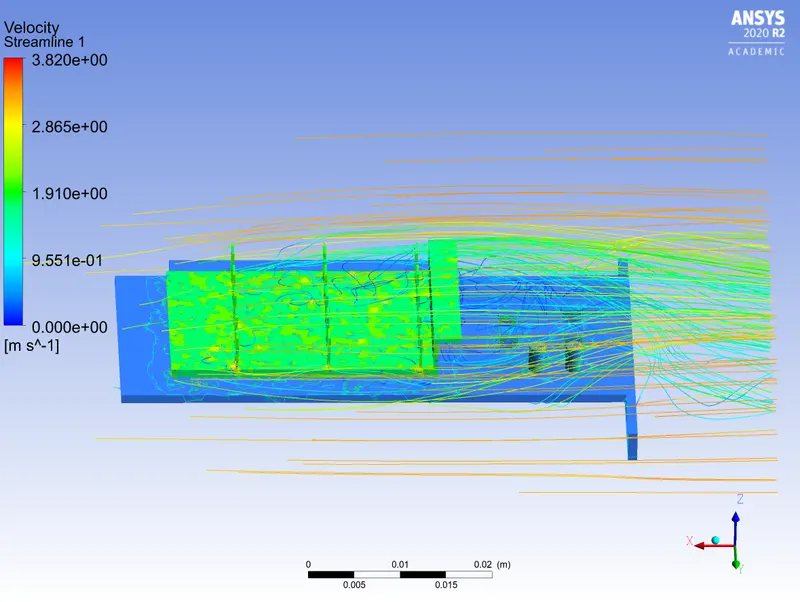
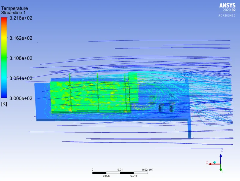
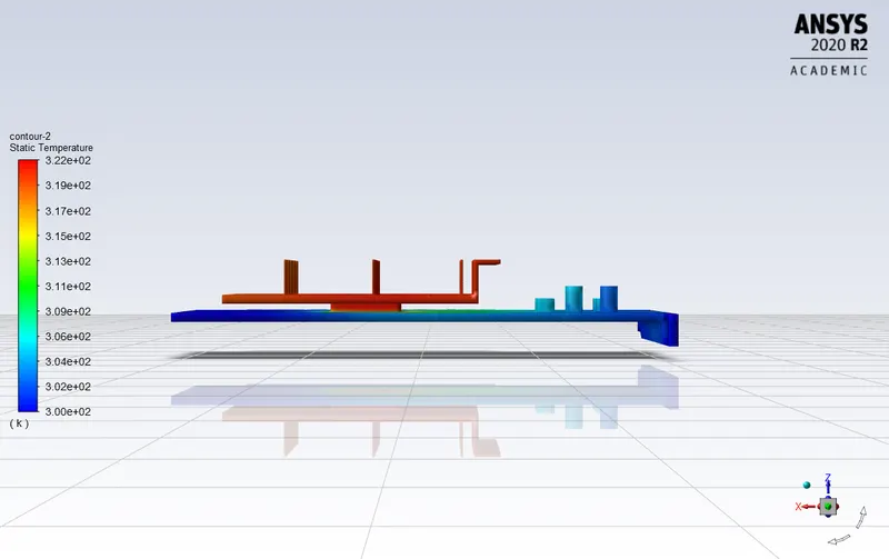
CASE 2: Refined mesh, inlet velocity 3 m/s (materials have been defined as above)
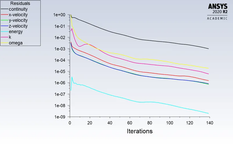
below is the graph of the residuals, we can see that the solution has converged (convergence criteria has been specified as the default values )
velocity streamlines(with wall heat transfer coefficient)
temperature streamlines(with wall heat transfer coefficent )
Temperature contours
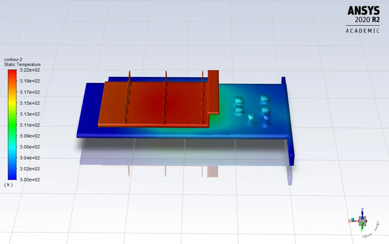
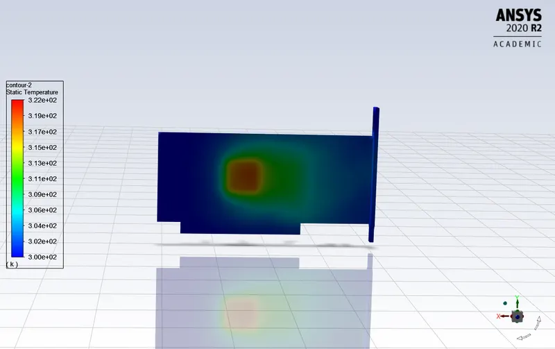
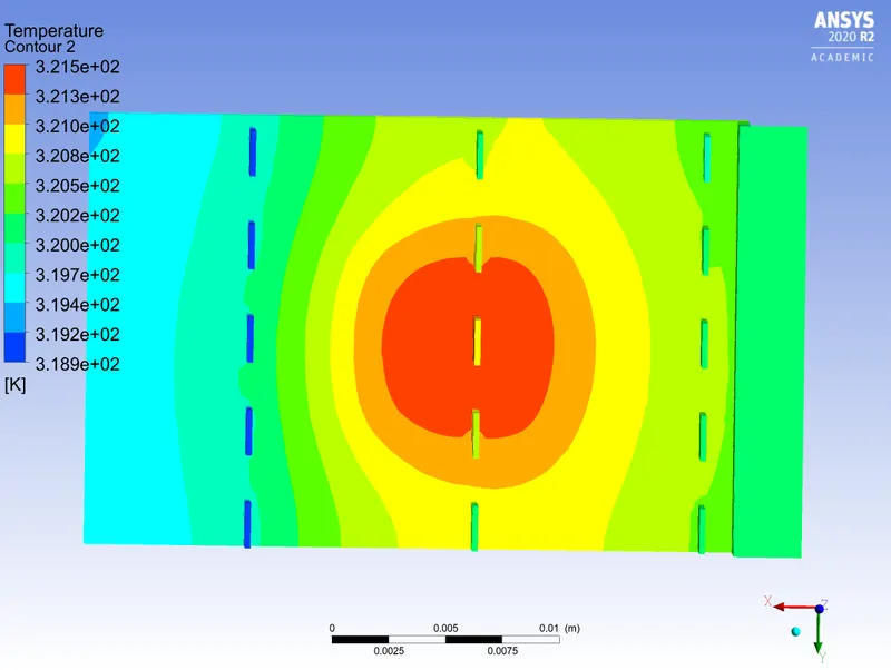
Local temperature contour for the fin
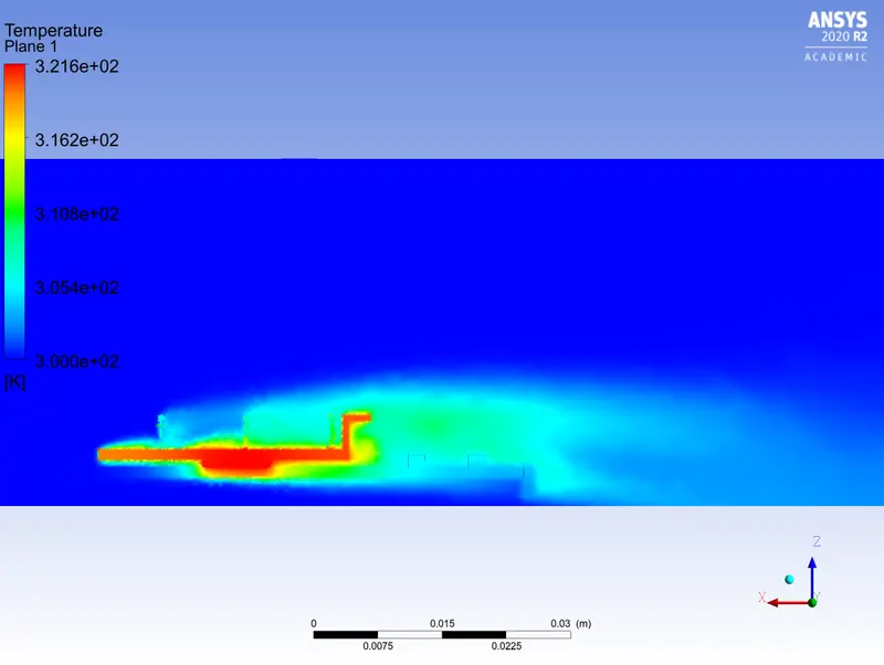
temperature plane contour
wall heat transfer coefficient
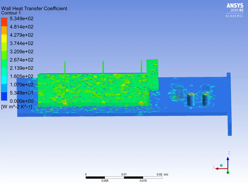
CASE 3: Refined mesh, inlet velocity 1 m/s (materials have been defined as above)
below is the graph of the residuals, we can see that the solution has converged (convergence criteria has been specified as the default values )
velocity streamlines (with wall heat transfer coefficent )
temperature streamlines(with wall heat transfer coefficent )
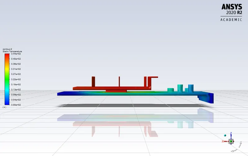
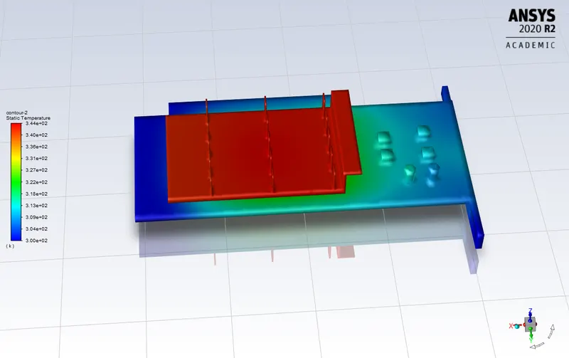
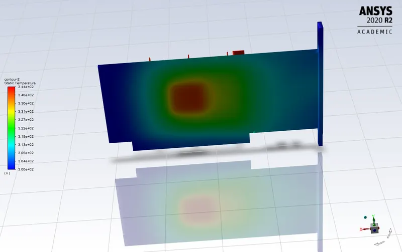
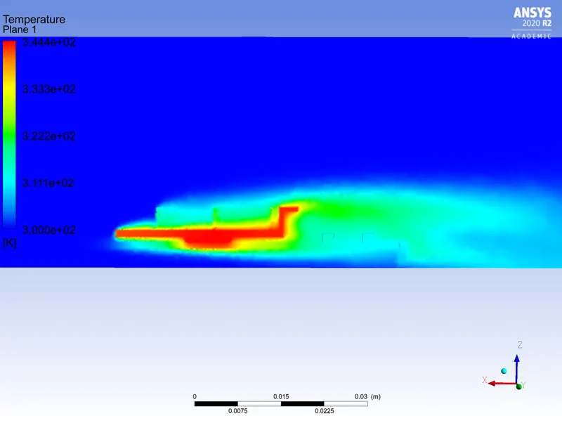
Temperature contours
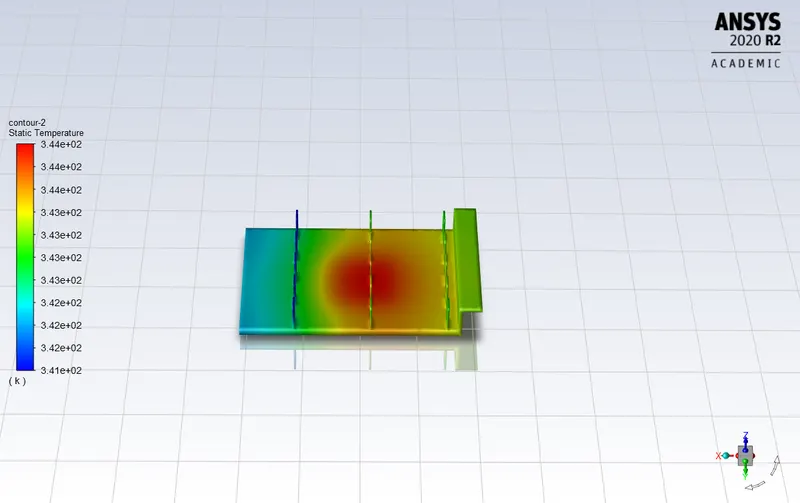
Local temperature contour for the fin
temperature plane contour
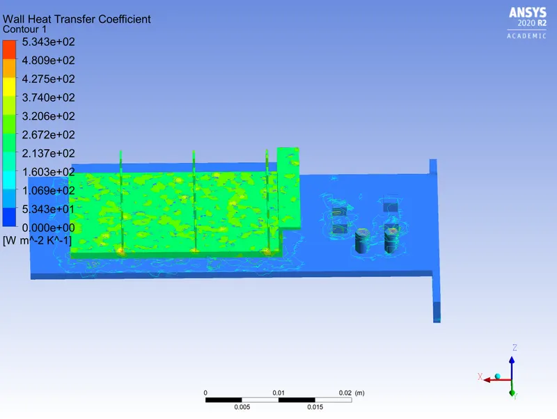
wall heat transfer coefficient
CONCLUSIONS:
| Sl No | Inlet Velocity(m/s) | Max temperature attained (K) | Max Velocity attained(M/s) | Max wall heat transfer coefficent |
| 1 | 5 | 316 | 6.3 | 5.37 |
| 2 | 3 | 322 | 3.8 | 5.349 |
| 3 | 1 | 344 | 1.16 | 5.343 |
- The CHT analysis was carried out successfully
- We can see from the temperature contour of the fins how the velocity affects the graphics card, lower velocity higher the temperature of the fins
- We can see that there is not much drastic change in the wall heat transfer coefficients.
- Wall heat transfer coefficients is majorly affected by the mesh size selected.
- The PCB board does not conduct away much heat and majority of the cooling work is done by the fins.
- Inlet air velocity and temperature plays an important role in the max temperature of the graphics card.