Solving the steady and unsteady 2D heat conduction problem (MATLAB)
AIM:
to solve the 2D steady and unsteady heat conduction problem.
OBJECTIVE:
to conduct the
- Steady state analysis
- Explicit Transient State Analysis
- Implicit Transient State Analysis
implementing the following methods for solving implicit equations.
- Jacobi
- Gauss-seidel
- Successive over-relaxation
THEORY:
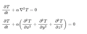
The 2D heat conduction equation is as follows
Steady state analysis:
When we assume steady state, we take the time derivate to be zero ie

the equation can therefore be written as
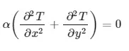
when we discretize the above equation in the second order derivative, central difference scheme we get

the above can be solved using the various iterative solvers
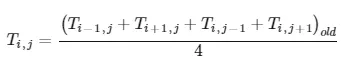
1) Jacobian
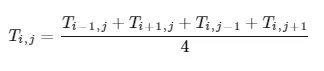
2)Gauss siedal method
3) Successive over-relaxation.
where w is the relaxation factor, the selection of the relaxation factor is important, if wis less than 1 the system is said to be underrelaxed, if greater than 1 the solution is said to be over relaxed. It is not good to take a really high value of w as this leads to the number of iterations performed increasing drastically.
Explicit transient analysis:
The heat conduction equation is

where i,j represent the node points

we use time marching to determine the answer.
Implicit transient anlysis:
The temperature varies with the variation in time node n

where n+1 is the next time step and n is the current time step.and k1 and k2 are as given below
k1=alpha*(dt/dx^2);
k2=alpha*(dt/dy^2);
cfl= k1+k1<=0.5;
if the cfl condition is not met the solution will blow up.
CODE:
steady state heat conduction.
%steady state analysis
%printing the output using all iterative methods
close all
clear all
clc

%inputs
l=1;
n=11; % defining the number of nodes
t_t=600;%k
t_b=900;%k
t_l=400;%k
t_r=800; %k
t=302*(ones(n)); %initialising t matrix to room temp values
%putting boundary conditions in t matrix
t(:,1)=t_l;
t(:,end)=t_r;
t(1,:)=t_t;
t(end,:)=t_b;
told=t;
tog=t;
tolerence=0.0001;


x=linspace(0,l,n);
y=x;
dx=x(2)-x(1);
dy=y(2)-y(1);
k=(2*(dx^2+dy^2))/(dx^2*dy^2);
[X Y]= meshgrid(x,y);
error=1;
error1=1;
error2=1;
counter=1;
w=1.1;

tic

%steady state
%gauss-seidal method
%convergence loop
while error >tolerence
    for i=2:n-1
        for j=2:n-1

            figure(1)% to print the gauss- seidal method
            l_r= (t(i-1,j)+t(i+1,j))/(k*dx^2);
            t_to_b= (t(i,j-1)+t(i,j+1))/(k*dy^2);
            t(i,j)=l_r+t_to_b;


        end

    end
    error=max(max(abs(told-t)));
     told=t;
    contourf(X,Y,t);
    xlabel('x Spatial');
    ylabel('y Spatial');
    axis ij;

     counter=counter+1;

end
h1=toc;
str1= sprintf('steady state gauss seidal method, iterations= %d ;time= %d',counter,h1);
title(str1);
t=tog;
told=tog;
counter=1;
tic
%jacobian method
%convergence loop
while error1 >tolerence
    for i=2:n-1
        for j=2:n-1

            figure(2)% to print the jacobian method
            l_r= (told(i-1,j)+told(i+1,j))/(k*dx^2);
            t_to_b= (told(i,j-1)+told(i,j+1))/(k*dy^2);
            t(i,j)=l_r+t_to_b;

        end

    end
    error1=max(max(abs(t-told)));
    told=t;
    contourf(X,Y,t);
   xlabel('x Spatial');
   ylabel('y Spatial');
    axis ij;

     counter=counter+1;

end
h2=toc;
str2= sprintf('steady state jacobian method, iterations= %d ;time= %d',counter,h2);
title(str2);

t=tog;
told=tog;
counter=1;
tic

%successive over-relaxation method
%convergence loop
while error2 >tolerence
    for i=2:n-1
        for j=2:n-1

            figure(3)% to print the successive over-relaxation method
            l_r= (t(i-1,j)+t(i+1,j))/(k*dx^2);
            t_to_b= (t(i,j-1)+t(i,j+1))/(k*dy^2);
           temporary1=w*(l_r+t_to_b);
            temporary2=(1-w)*told(i,j);
            t(i,j)=temporary1+temporary2;
        end

    end
    error2=max(max(abs(t-told)));
    told=t;
    contourf(X,Y,t);
    xlabel('x Spatial');
    ylabel('y Spatial');
    axis ij;

     counter=counter+1;

end
h3=toc;
str3= sprintf('steady state successive over-relaxation method, iterations= %d ;time= %d',counter,h3);
title(str3);
OUTPUT:
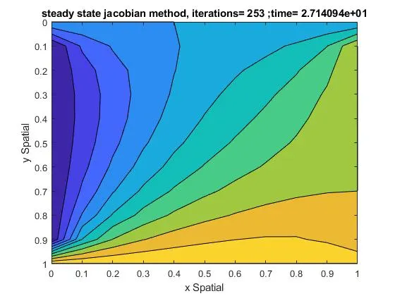
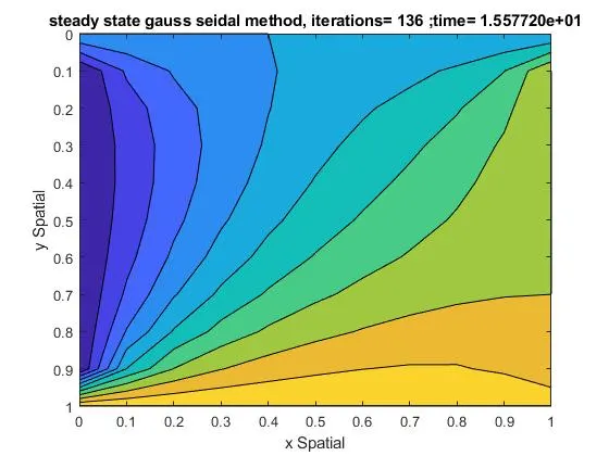
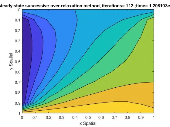
CONCLUSION
the jacobian method takes 253 iterations to complete;
the gauss-seidal method takes 136 iterations to complete;
the SOR method takes 112 iterations to complete
SOR gives the least computational time to solve the problem.
CODE:
The code for explicit transient heat conduction is given below
%transient state, explicit.
%printing the output using all iterative methods
close all
clear all
clc

%inputs
l=1;
n=11; % defining the number of nodes
t_t=600;%k
t_b=900;%k
t_l=400;%k
t_r=800; %k
t=302*(ones(n)); %initialising t matrix to room temp values
%putting boundary conditions in t matrix
t(:,1)=t_l;
t(:,end)=t_r;
t(1,:)=t_t;
t(end,:)=t_b;
told=t;

tolerence=0.0001;

x=linspace(0,l,n);
y=x;
dx=x(2)-x(1);
dy=y(2)-y(1);
dt=1.6667e-03;
[X Y]= meshgrid(x,y);
error=1;
counter=1;
alpha=1.5;
k1=alpha*(dt/dx^2);
k2=alpha*(dt/dy^2);
cfl= k1+k2

tic


%convergence loop
%time marching
while error >tolerence
    for i=2:n-1
        for j=2:n-1

            figure(1)
            l_r= (told(i-1,j)-2*told(i,j)+told(i+1,j));
            t_to_b= (told(i,j-1)-2*told(i,j)+told(i,j+1));
            t(i,j)=told(i,j)+(l_r*k1)+(t_to_b*k2);

        end

    end
    error=max(max(abs(told-t)));
     told=t;
    contourf(X,Y,t);
    grid on;
    xlabel('x Spatial');
    ylabel('y Spatial');
    axis ij;

     counter=counter+1;

end
h1=toc;
str1= sprintf('transient explicit method, iterations= %d ;time= %d',counter,h1);
title(str1);
OUTPUT:
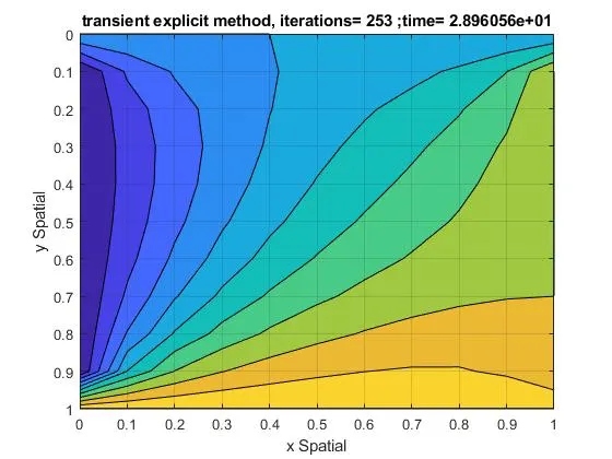
CONCLUSION:
As this is a time marching solution we can see that this depends on the value of dt if the value of dt does not satisfy the cfl criteria the solution will blow up.
CODE:
the code for the implicit transient heat conduction is given below
%transient implicit analysis
%printing the output using all iterative methods
close all
clear all
clc

%inputs
l=1;
n=11; % defining the number of nodes
t_t=600;%k
t_b=900;%k
t_l=400;%k
t_r=800; %k
t=302*(ones(n)); %initialising t matrix to room temp values
%putting boundary conditions in t matrix
t(:,1)=t_l;
t(:,end)=t_r;
t(1,:)=t_t;
t(end,:)=t_b;
told=t;
tog=t;
tog2=t;
tolerence=0.0001;
dt=1.6667e-03;
w=1.1;

x=linspace(0,l,n);
y=x;
dx=x(2)-x(1);
dy=y(2)-y(1);
k=(2*(dx^2+dy^2))/(dx^2*dy^2);
[X Y]= meshgrid(x,y);
error=1;
error1=1;
error2=1;
counter=1;
alpha=1.5;
k1=alpha*(dt/dx^2);
k2=alpha*(dt/dy^2);
cfl= k1+k2;


tic


%gauss-seidal method
%convergence loop
for m=1:1400
    error=1;
while error >tolerence
    for i=2:n-1
        for j=2:n-1


            term1=1/(1+(k1*2)+(k2*2));
            term2= k1*term1;
            term3= k2*term1;
            l_r= (t(i-1,j)+told(i+1,j));
            t_to_b= (t(i,j-1)+told(i,j+1));
            t(i,j)=(tog(i,j)*term1)+(l_r*term2)+(t_to_b*term3);


        end

    end
    error=max(max(abs(told-t)));
     told=t;


     counter=counter+1;

end
tog=t;
end
figure(1)% to print the gauss- seidal method
 contourf(X,Y,t);
    xlabel('x Spatial');
    ylabel('y Spatial');
    axis ij;

h1=toc;
str1= sprintf('transient implicit gauss seidal method, iterations= %d ;time= %d',counter,h1);
title(str1);

t=tog2;
told=tog2;
tog=tog2;
counter=1;
tic
%jacobian method
for m=1:1400
    error1=1;
%convergence loop
while error1 >tolerence
    for i=2:n-1
        for j=2:n-1

            term1=1/(1+(k1*2)+(k2*2));
            term2= k1*term1;
            term3= k2*term1;
            l_r= (told(i-1,j)+told(i+1,j));
            t_to_b= (told(i,j-1)+told(i,j+1));
            t(i,j)=(tog(i,j)*term1)+(l_r*term2)+(t_to_b*term3);
        end

    end
    error1=max(max(abs(told-t)));
     told=t;
     counter=counter+1;
end
tog=t;
end
figure(2)% to print the jacobi method
 contourf(X,Y,t);
    xlabel('x Spatial');
    ylabel('y Spatial');
    axis ij;

h2=toc;
str2= sprintf('transient implicit jacobian method, iterations= %d ;time= %d',counter,h2);
title(str2);

t=tog2;
told=tog2;
tog=tog2;
counter=1;
tic
 %successive over-relaxation method
for m=1:1400
    error2=1;
% %convergence loop
while error2 >tolerence
    for i=2:n-1
        for j=2:n-1

            term1=1/(1+(k1*2)+(k2*2));
            term2= k1*term1;
            term3= k2*term1;
            l_r= (t(i-1,j)+told(i+1,j));
            t_to_b= (t(i,j-1)+told(i,j+1));
           temporary1=w*((tog(i,j)*term1)+(l_r*term2)+(t_to_b*term3));
           temporary2=(1-w)*told(i,j);
           t(i,j)=temporary1+temporary2;
        end

    end
    error2=max(max(abs(t-told)));
    told=t;
    counter=counter+1;

end
tog=t;
end
figure(3)% to print the SOR method
 contourf(X,Y,t);
    xlabel('x Spatial');
    ylabel('y Spatial');
    axis ij;

h3=toc;
str2= sprintf('transient implicit SOR method, iterations= %d ;time= %d',counter,h3);
title(str2);
OUTPUT:
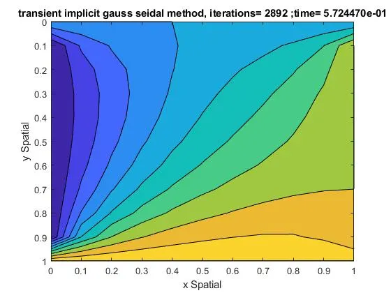
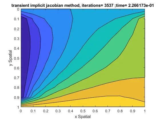
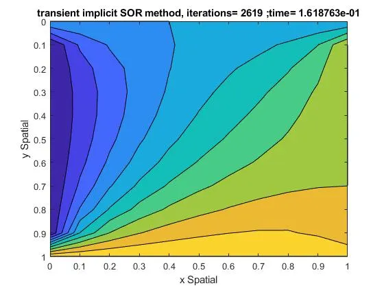
CONCLUSION:
the logic used for the implicit function causes a lot more iterations to be performed,
the jacobian method takes 3537 iterations to complete;
the gauss-seidal method takes 2892 iterations to complete;
the SOR method takes 2619 iterations to complete
SOR gives the least computational time to solve the problem.but if tghe value of w is changed the number of iterations it takes for the solution to converge is also changed, 1.1 gives the best answer.