Week 3 - Taylor table method and Matlab code

AIM:

To Derive the following 4th order approximations of the second-order derivative of a given continuous function using taylors table method.

OBJECTIVE:

1. To calculate the taylor series coefficients for central difference,skewed right side difference and skewed left side difference
2. Compare the analytical derivative to the 3 numerical approximates derived.
3. Provide a plot that compares the absolute error between the above-mentioned schemes

THEORY:

1. right skewed differencing scheme
   
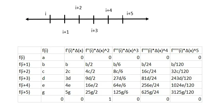
   The unknows are solved with the following matlab code
   

   % rightskewed scheme
   a= [1 1 1 1 1 1;0 1 2 3 4 5;0 1/2 2 9/2 8 25/2;0 1/6 8/6 27/6 64/6 125/6;0 1/24 16/24 81/24 256/24 625/24; 0 1/120 32/120 243/120 1024/120 3125/120]
   b= [0; 0; 1; 0; 0; 0]
   
   format rat
   r= (linsolve(a,b))​

   
   this will output the coefficients
   
   15/4
   -77/6
   107/6
   -13
   61/12
   -5/6
   
   
2. left skewed differencing scheme
   
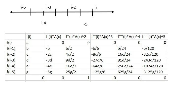
   The unknows are solved with the following matlab code
   

   % left skewed scheme
   a= [1 1 1 1 1 1;0 1 2 3 4 5;0 1/2 2 9/2 8 25/2;0 1/6 8/6 27/6 64/6 125/6;0 1/24 16/24 81/24 256/24 625/24; 0 1/120 32/120 243/120 1024/120 3125/120]
   b= [0; 0; 1; 0; 0; 0]
   
   format rat
   r= (linsolve(a,b))​

   this will output the coefficients
   
   15/4
   -77/6
   107/6
   -13
   61/12
   -5/6
   
   
3. central differencing scheme
   
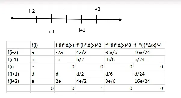
   The unknows are solved with the following matlab code
   

       % central differencing scheme
       a= [1 1 1 1 1 ;-2 -1 0 1 2;2 1/2 0 1/2 2;-8/6 -1/6 0 1/6 8/6;16/24 1/24 0 1/24 16/24] 
       b= [0; 0; 1; 0; 0]
   
       format rat
       r= (linsolve(a,b))​

   this will output the coefficients
   
   -1/12
   4/3
   -5/2
   4/3
   -1/12

CODE:

The following code was written on MATLAB:

clear all 
close all 
clc

dx=linspace(pi/4000,pi/40,20);
x= pi/4;
%the function is (e^x)*cos(x)
analytical_derivative = -2*exp(x)*sin(x)

for i=1:length(dx)
 %taylor series function at various nodes 
 a(i)=(exp(x-(5*dx(i)))*cos(x-(5*dx(i))));
 b(i)=(exp(x-(4*dx(i)))*cos(x-(4*dx(i))));
 c(i)=(exp(x-(3*dx(i)))*cos(x-(3*dx(i))));
 d(i)=(exp(x-(2*dx(i)))*cos(x-(2*dx(i))));
 e(i)=(exp(x-(1*dx(i)))*cos(x-(1*dx(i))));
 f(i)=(exp(x))*(cos(x));
 g(i)=(exp(x+(1*dx(i)))*cos(x+(1*dx(i))));
 h(i)=(exp(x+(2*dx(i)))*cos(x+(2*dx(i))));
 I(i)=(exp(x+(3*dx(i)))*cos(x+(3*dx(i))));
 j(i)=(exp(x+(4*dx(i)))*cos(x+(4*dx(i))));
 k(i)=(exp(x+(5*dx(i)))*cos(x+(5*dx(i))));
  
%formulae for various taylor series function 
%central difference scheme 
CDS(i)=((-d(i))+16*e(i)-30*f(i)+(16*g(i))-h(i))/(12*dx(i)^2);

%right skewed difference scheme
RSDS(i)=(45*f(i)-154*g(i)+214*h(i)-156*I(i)+61*j(i)-10*k(i))/(12*dx(i)^2);

%left skewed difference scheme
LSDS(i)=(45*f(i)-154*e(i)+214*d(i)-156*c(i)+61*b(i)-10*a(i))/(12*dx(i)^2);

%calculating error 
error_CDS(i)=abs(CDS(i)-analytical_derivative);
error_RSDS(i)=abs(RSDS(i)-analytical_derivative);
error_LSDS(i)=abs(LSDS(i)-analytical_derivative);
end

%plotting
figure(1)
    
    loglog(dx,error_CDS); % using loglog to make sense of the error values 
    hold on
    loglog(dx,error_RSDS);
    loglog(dx,error_LSDS);
    legend('central difference scheme error','right skewed difference scheme error','left skewed difference scheme error')
    xlabel('values of dx');
    ylabel('error')
    
    
    

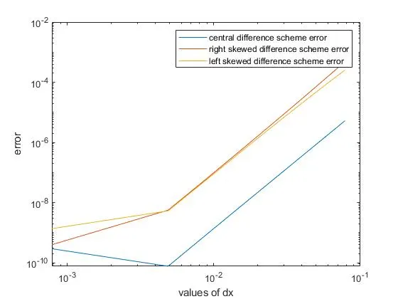
OUTPUT:

CONCLUSION:

we can see that the descritizantion errors keep on decreasing as the values of dx become smaller but only upto a point. after this point the roundoff errors take over and the errors being to rise again.
we can also see that the central difference scheme is generally more accurate as compared to the right and left skewed difference schemes.