Week 9 - FVM Literature Review

AIM :

To describe the need for discretization, interpolation schemes and flux limiters in FVm

THEORY:

In fluid dynamics the 3 main methods to solve the PDE's of the navier stokes equation by converting them into algebraic forms are

1. Finite Difference Method
2. Finite Volume Method
3. Finite Element Method

Finite Difference Method:

finite-difference methods (FDM) are a class of numerical techniques for solving differential equations by approximating derivatives with finite differences. Both the spatial domain and time interval (if applicable) are discretized, or broken into a finite number of steps, and the value of the solution at these discrete points is approximated by solving algebraic equations containing finite differences and values from nearby points.
Finite difference methods convert ordinary differential equations (ODE) or partial differential equations (PDE), which may be nonlinear, into a system of linear equations that can be solved by matrix algebra techniques.

Finite Volume Method:

The finite volume method (FVM) is a method for representing and evaluating partial differential equations in the form of algebraic equations.^[1] In the finite volume method, volume integrals in a partial differential equation that contain a divergence term are converted to surface integrals, using the divergence theorem. These terms are then evaluated as fluxes at the surfaces of each finite volume. Because the flux entering a given volume is identical to that leaving the adjacent volume, these methods are conservative. Another advantage of the finite volume method is that it is easily formulated to allow for unstructured meshes
In contrast to FDM a finite volume method evaluates exact expressions for the average value of the solution over some volume, and uses this data to construct approximations of the solution within cells.

the FVM consists of 3 main steps

1. Grid generation
2. Discretization
3. Solution of equations

Finite Element Method:

The finite element method (FEM) is the most widely used method for solving problems of engineering and mathematical models.The FEM is a particular numerical method for solving partial differential equations in two or three space variables (i.e., some boundary value problems). To solve a problem, the FEM subdivides a large system into smaller, simpler parts that are called finite elements. This is achieved by a particular space discretization in the space dimensions, which is implemented by the construction of a mesh of the object: the numerical domain for the solution, which has a finite number of points.

Main differences between FVM and FDM

1)Simply put, FDM is a differential scheme, that is approximation of a taylor series expansion. You try to write the first order, second order differential in terms of difference between two point values.
Finite Volume method is an integral scheme.

2) FDM may bring in some approximation error.In FVM since you are integrating across the area, chance of error is minimized.

3)FDM schemes are faster
FVM schemes are slightly slower

4)in FDM mesh is irregular, in FVM, the mesh is continuous

5) in FDM the values are calculated at every node, in FVM the values are calculated for each cell

6)for complex profiles the FVM is prefered, FDM is not prefered

let us futher discuss the 3 main steps of FVM

• Grid generation:
  The basic idea of FVM is to divide domain Ω into a set of disjoint finite volumes and apply the conservation law on each finite volume. The division of Ω gives rise to the mesh or grid. The mesh can consist of different types of cells, e.g., triangular and quadrilateral cells in 2-D. Such a mesh is called hybrid mesh.
  Once a mesh has been formed, we have to create the finite volumes on which the conservation law will be applied. This can be done in two ways, depending on where the solution is stored.
  1)If the solution is stored at the center of each Ωi, then Ωi itself is the finite volume or cell, Ci = Ωi. This gives rise to the cell-centered
  finite volume scheme.
  2) If the solution is stored at the vertices of the mesh, then around each vertex i we have to construct a cell Ci. This gives rise to the
  vertex-centered finite volume scheme.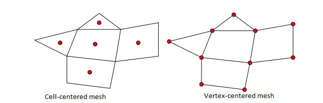
  
• Discretization:
  The key step of the finite volume method is the integration of the governing equation (or equations) over a control volume to yield a discretised equation at its nodal point P. in most simple cases we are able to use a basic central differencing scheme.a very attractive feature of the finite volume method that the discretised equation has a clear physical interpretation. The diffusive flux of φ leaving the east face minus the diffusive flux of φ entering the west face is equal to the generation of φ, i.e. it constitutes a balance equation for φ over the control volume.
  The failure of central differencing in certain cases involving combined convection and diffusion forces us to take a more in-depth look at the properties of discretisation schemes.the discretisation scheme has certain fundamental properties. The most important ones are:
  
  • Conservativeness- To ensure conservation of φ for the whole solution domain the flux of φ leaving a control volume across a certain face must be equal to the flux of φ entering the adjacent control volume through the same face. To achieve this the flux through a common face must be represented in a consistent manner by one and the same expression in adjacent control volumes.
  • Boundedness-Diagonal dominance is a desirable feature for satisfying the ‘boundedness’ criterion. This states that in the absence of sources the internal nodal values of property φ should be bounded by its boundary values.
  • Transportiveness-For fluid flow, transportiveness describes the influence on the upstream node on the downstream node.
  
  the central differencing scheme is not perfect for all cfd problems therefore a few of the various other schemes that can be used are
  1)upwind differencing scheme :
  In computational physics, upwind schemes denote a class of numerical discretization methods for solving hyperbolic partial differential equations. Upwind schemes use an adaptive or solution-sensitive finite difference stencil to numerically simulate the direction of propagation of information in a flow field. The upwind schemes attempt to discretize hyperbolic partial differential equations by using differencing biased in the direction determined by the sign of the characteristic speeds
  they can be represented by the general form
  aP φP = aW φW + aE φ
  with the central term being
  aP = aW + aE + (Fe − Fw)
  
  2)the hybrid differencing scheme:
  Hybrid difference scheme is a method used in the numerical solution for convection-diffusion problems.

  

  Where, is density, is the velocity vector, is the diffusion coefficient and is the source term. In this equation property, can be temperature, internal energy or component of velocity vector in x, y and z directions.

  
  3)the power law scheme:
  The power-law differencing scheme is a more accurate approximation to the one-dimensional exact solution and produces better results than the hybrid scheme. In this scheme diffusion is set to zero whencell Pe exceeds 10. If 0 < Pe < 10 the flux is evaluated by using a polynomial expression.
  For example, the net flux per unit area at the west control volume face is evaluated using
  qw = Fw[φW − βw(φP − φW)] for 0 < Pe < 10 (5.44a)
  where βw = (1 − 0.1Pew)^5/Pew
  and
  qw = FwφW for Pe > 10
  
  4) Quadratic upwind differencing scheme:
  uses a three-point upstream-weighted quadratic interpolation for cell face values. The face value of φ is obtained from a quadratic function passing through two bracketing nodes (on each side of the face) and a node on the upstream side
  This is now written in the standard form for discretised equations:
  aPφP = aW φW + aEφE + aWW φWW
  where
  
  5) TVD Scheme:
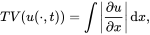
  The class of TVD (total variation diminishing) schemes has been specially formulated to achieve oscillation-free solutions and has proved to be useful in CFD calculations. TVD is a property used in the discretisation of equations governing time-dependent gas dynamics problems. More recently, schemes with this property have also become popular in general-purpose CFD solvers.
  

  In systems described by partial differential equations, such as the following hyperbolic advection equation,

  

  the total variation (TV) is given by

  

  and the total variation for the discrete case is,

  

  where .

  A numerical method is said to be total variation diminishing (TVD) if,

  

  
  
  
• Solution to the equation:
  Discretised equations of the form must be set up at each of the nodal points in order to solve a problem. For control volumes that are adjacent to the domain boundaries the general discretised equation is modified to incorporate boundary conditions. The resulting system of linear algebraic equations is then solved to obtain the distribution of the property φ at nodal points. Any suitable matrix solution technique may be enlisted for this task.

FLUX LIMITER:

Flux limiters are used in high resolution schemes, described by partial differential equations (PDE's). They are used in high resolution schemes, to avoid the spurious oscillations (wiggles) that would otherwise occur with high order spatial discretization schemes due to shocks, discontinuities or sharp changes in the solution domain. Use of flux limiters, together with an appropriate high resolution scheme, make the solutions total variation diminishing (TVD).The main idea behind the construction of flux limiter schemes is to limit the spatial derivatives to realistic values

Consider the 1D semi-discrete scheme below,

where, and represent edge fluxes for the ith cell. If these edge fluxes can be represented by low and high resolution schemes, then a flux limiter can switch between these schemes depending upon the gradients close to the particular cell, as follows,

,

,

where

low resolution flux,

high resolution flux,

flux limiter function,

and represents the ratio of successive gradients on the solution mesh, i.e.,

.

The limiter function is constrained to be greater than or equal to zero, i.e.. Therefore, when the limiter is equal to zero (sharp gradient, opposite slopes or zero gradient), the flux is represented by a low resolution scheme. Similarly, when the limiter is equal to 1 (smooth solution), it is represented by a high resolution scheme. The various limiters have differing switching characteristics and are selected according to the particular problem and solution scheme. No particular limiter has been found to work well for all problems, and a particular choice is usually made on a trial and error basis.