Simulation of Flow through a pipe in OpenFoam: part 2 (OpenFoam MATLAB)
AIM:
To simulate the laminar flow of water through a pipe.
OBJECTIVE:
- Write a program in Matlab that can generate the computational mesh automatically for any wedge angle and grading scheme
- For a baseline mesh, show that the velocity profile matches with the Hagen poiseuille's equation
- Show that the velocity profile is fully developed
- Post process velocity and shear stress
- You should obtain results for the pipe flow with symmetry BC
- Angles to test 10,25,45
THEORY:
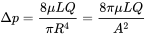
Hagen–Poiseuille equation:
In nonideal fluid dynamics, the Hagen–Poiseuille equation, is a physical law that gives the pressure drop in an incompressible and Newtonian fluid in laminar flow flowing through a long cylindrical pipe of constant cross section. It can be successfully applied to air flow in lung alveoli, or the flow through a drinking straw or through a hypodermic needle.
REYNOLDS Number:
The Reynolds number (Re) helps predict flow patterns in different fluid flow situations. At low Reynolds numbers, flows tend to be dominated by laminar (sheet-like) flow, while at high Reynolds numbers flows tend to be turbulent. The turbulence results from differences in the fluid's speed and direction, which may sometimes intersect or even move counter to the overall direction of the flow (eddy currents).Reynolds numbers are an important dimensionless quantity in fluid mechanics.
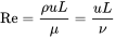
Re ≲ 2300 laminar flow
2300 ≲ Re ≲ 4000 transitional flow
Re ≳ 4000 turbulent flow
Enterance length:
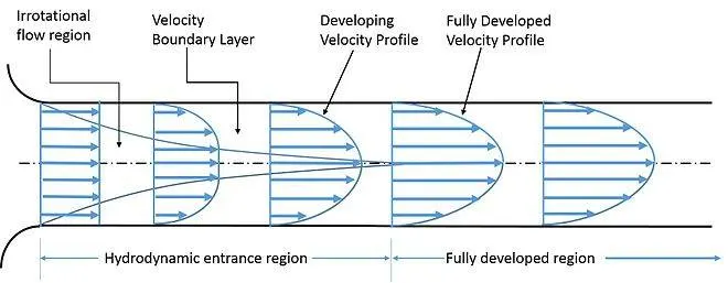
Consider a fluid entering a circular pipe at a uniform velocity. Because of the no-slip condition, the fluid particles in the layer in contact with the wall of the pipe come to a complete stop. This layer also causes the fluid particles in the adjacent layers to slow down gradually as a result of friction. To make up for this velocity reduction, the velocity of the fluid at the midsection of the pipe has to increase to keep the mass flow rate through the pipe constant. As a result, a velocity gradient develops along the pipe.
The region of the flow in which the effects of the viscous shearing forces caused by fluid viscosity are felt is called the velocity boundary layer or just the boundary layer.The thickness of this boundary layer increases in the flow direction until the boundary layer reaches the pipe center and thus fills the entire pipe.The region from the pipe inlet to the point at which the velocity profile is fully developed is called the hydrodynamic entrance region and the length of this region is called the hydrodynamic entry length Lh.
Lh, (laminar)/D≅ 0.05Re
the velocity profile in fully developed laminar flow in a pipe is parabolic with a maximum at the centerline and a minimum (zero) at the pipe wall.
u(r) = 2Vavg(1 − r^2/R^2)
where r = radial distance from centerline
R= radius of the pipe.
from this we can see that max velocity is given by
u_max=2*Vavg
Pressure loss:
A quantity of interest in the analysis of pipe flow is the pressure drop ΔP since it is directly related to the power requirements of the fan or pump to
maintain flow. We note that dP/dx = constant, and integrating from x = x1 where the pressure is P1 to x = x1 + L where the pressure is P2 gives
dP/dx = (P2 − P1)/L
In the analysis of piping systems, pressure losses are commonly expressed in terms of the equivalent fluid column height, called the head loss hL
hL = ΔPl/ρg
why wedge ?
Applied in pairs to 2-D rotationally symmetric cases to represent planes in the swirl direction.since the laminar flow through a pipe is axisymmetric we can convert the circular cross-section into an arc, this will greatly save on the computation time required to simulate this problem.
{
    type            wedge;
    ...
}
why symmetryPlane?
the symmetry plane boundary condition, Applies to planar patches to represent a symmetry condition.since the laminar flow through a pipe is axisymmetric we can convert the circular cross-section into an arc, this will greatly save on the computation time required to simulate this problem.
{
    type            symmetryPlane;
    ...
}
WHY icoFoam ?
we choose the icofoam solver because the flow we are simulating is of an incompressiable, transient, viscous and laminar nature and the icofoam solver is easy to use and modify, to suit our needs
ASSUMPTIONS:
pipe diameter = 0.02 m
wedge angle =4
reynolds number = 2100
kinematic viscosity = 0.000001 m^2/s
CODE:
the following is the matlab code to create the blockMeshDict file
clear all
close all
clc

re=2100;
d=0.02;
r=d/2;
theta= input('enter the value of theta angle (preferably less than 5 degrees)');
l_e=0.06*re*d; % entry length
l=l_e+0.5;
h=r*sind(theta/2);
v=r*cosd(theta/2);
%finding the vertices
v0=[0 0 0];
v1=[-h v 0];
v2=[h v 0];
v3=[0 0 l];
v4=[-h v l];
v5=[h v l];

f= fopen('blockMeshDict3.txt','w');

fprintf(f,'%sn','/*--------------------------------*- C++ -*----------------------------------*');
fprintf(f,'%sn','  =========                 |');
fprintf(f,'%sn','  \      /  F ield         | OpenFOAM: The Open Source CFD Toolbox');
fprintf(f,'%sn','   \    /   O peration     | Website:  https://openfoam.org');
fprintf(f,'%sn','    \  /    A nd           | Version:  8');
fprintf(f,'%sn','     \/     M anipulation  |');
fprintf(f,'%sn','*---------------------------------------------------------------------------*/');
fprintf(f,'%sn','FoamFile');
fprintf(f,'%sn','{');
fprintf(f,'%sn','    version     2.0;');
fprintf(f,'%sn','    format      ascii;');
fprintf(f,'%sn','    class       dictionary;');
fprintf(f,'%sn','    object      blockMeshDict;');
fprintf(f,'%sn','}');
fprintf(f,'%sn','// * * * * * * * * * * * * * * * * * * * * * * * * * * * * * * * * * * * * * //');
fprintf(f,'%sn','');
fprintf(f,'%sn','convertToMeters 1;');
fprintf(f,'%sn','');
fprintf(f,'%sn','vertices');
fprintf(f,'%sn','(');
fprintf(f,'    (%f %f %f)n',v0(1),v0(2),v0(3));
fprintf(f,'    (%f %f %f)n',v1(1),v1(2),v1(3));
fprintf(f,'    (%f %f %f)n',v2(1),v2(2),v2(3));
fprintf(f,'    (%f %f %f)n',v3(1),v3(2),v3(3));
fprintf(f,'    (%f %f %f)n',v4(1),v4(2),v4(3));
fprintf(f,'    (%f %f %f)n',v5(1),v5(2),v5(3));

fprintf(f,'%sn',');');
fprintf(f,'%sn','');
fprintf(f,'%sn','blocks');
fprintf(f,'%sn','(');
fprintf(f,'%sn','    hex (0 2 1 0 3 5 4 3) (20 1 500) simpleGrading (1 1 1)');
fprintf(f,'%sn',');');
fprintf(f,'%sn','');
fprintf(f,'%sn','edges');
fprintf(f,'%sn','(');
fprintf(f,'%sn','	arc 1 2 (0 0.01 0)');
fprintf(f,'%sn','	arc 4 5 (3 0.01 0)');
fprintf(f,'%sn',');');
fprintf(f,'%sn','');
fprintf(f,'%sn','boundary');
fprintf(f,'%sn','(');
fprintf(f,'%sn','    inlet');
fprintf(f,'%sn','    {');
fprintf(f,'%sn','        type patch;');
fprintf(f,'%sn','        faces');
fprintf(f,'%sn','        (');
fprintf(f,'%sn','            (0 0 1 2)');
fprintf(f,'%sn','        );');
fprintf(f,'%sn','    }');
fprintf(f,'%sn','    outlet');
fprintf(f,'%sn','    {');
fprintf(f,'%sn','        type patch;');
fprintf(f,'%sn','        faces');
fprintf(f,'%sn','        (');
fprintf(f,'%sn','            (3 5 4 3)');
fprintf(f,'%sn','        );');
fprintf(f,'%sn','    }');
fprintf(f,'%sn','    top');
fprintf(f,'%sn','    {');
fprintf(f,'%sn','        type wall;');
fprintf(f,'%sn','        faces');
fprintf(f,'%sn','        (');
fprintf(f,'%sn','            (1 4 5 2)');
fprintf(f,'%sn','        );');
fprintf(f,'%sn','    }');
fprintf(f,'%sn','    wedge1');
fprintf(f,'%sn','    {');
fprintf(f,'%sn','        type wedge;');
fprintf(f,'%sn','        faces');
fprintf(f,'%sn','        (');
fprintf(f,'%sn','            (0 2 5 3)');
fprintf(f,'%sn','        );');
fprintf(f,'%sn','    }');
fprintf(f,'%sn','    wedge2');
fprintf(f,'%sn','    {');
fprintf(f,'%sn','        type wedge;');
fprintf(f,'%sn','        faces');
fprintf(f,'%sn','        (');
fprintf(f,'%sn','            (0 3 4 1)');
fprintf(f,'%sn','        );');
fprintf(f,'%sn','    }');
fprintf(f,'%sn','    bot');
fprintf(f,'%sn','    {');
fprintf(f,'%sn','        type empty;');
fprintf(f,'%sn','        faces');
fprintf(f,'%sn','        (');
fprintf(f,'%sn','            (0 0 3 3)');
fprintf(f,'%sn','        );');
fprintf(f,'%sn','    }');
fprintf(f,'%sn',');');
fprintf(f,'%sn','');
fprintf(f,'%sn','mergePatchPairs');
fprintf(f,'%sn','(');
fprintf(f,'%sn',');');
fprintf(f,'%sn','');
fprintf(f,'%sn','// ************************************************************************* //');
The above code creates blockMeshDict files according to the angle inputed by the user.
One of the blockMeshDict files is shown below. this is for a wedge angle of 10 degrees
/*--------------------------------*- C++ -*----------------------------------*
  =========                 |
  \      /  F ield         | OpenFOAM: The Open Source CFD Toolbox
   \    /   O peration     | Website:  https://openfoam.org
    \  /    A nd           | Version:  8
     \/     M anipulation  |
*---------------------------------------------------------------------------*/
FoamFile
{
    version     2.0;
    format      ascii;
    class       dictionary;
    object      blockMeshDict;
}
// * * * * * * * * * * * * * * * * * * * * * * * * * * * * * * * * * * * * * //

convertToMeters 1;

vertices
(
    (0.000000 0.000000 0.000000)
    (-0.000872 0.009962 0.000000)
    (0.000872 0.009962 0.000000)
    (0.000000 0.000000 3.020000)
    (-0.000872 0.009962 3.020000)
    (0.000872 0.009962 3.020000)
);

blocks
(
    hex (0 2 1 0 3 5 4 3) (20 1 500) simpleGrading (1 1 1)
);

edges
(
	arc 1 2 (0 0.01 0)
	arc 4 5 (3 0.01 0)
);

boundary
(
    inlet
    {
        type patch;
        faces
        (
            (0 0 1 2)
        );
    }
    outlet
    {
        type patch;
        faces
        (
            (3 5 4 3)
        );
    }
    top
    {
        type wall;
        faces
        (
            (1 4 5 2)
        );
    }
    wedge1
    {
        type wedge;
        faces
        (
            (0 2 5 3)
        );
    }
    wedge2
    {
        type wedge;
        faces
        (
            (0 3 4 1)
        );
    }
    bot
    {
        type empty;
        faces
        (
            (0 0 3 3)
        );
    }
);

mergePatchPairs
(
);

// ************************************************************************* //
- The above matlab code takes a user defined wedge angle and uses that angle to calculate the vertices for the mesh.
- The entrance length is also calculated and 0.5 m is added to the value so as to be able to observe the fully developed region of the flow.
- The number of cells for the wedge is also defined. 500 along the z axis. 20along the x axis and 1 along the y axis, these values are taken as such due to the way the block has been defined
- Make note of the direction of the normal vector when defining the block and while defining the faces, in the block, the normal of the inlet and outlet point in the direction of the flow. when defining the faces the normals always point outward.
- The wedge boundaries are defined as wedge, which is predefined in openFoam
- The above code is for the wedge boundary condition when we need to simulate the symmetry condition we must replace 'wedge ' in the above code with 'symmetryPlane'
- v0 to v5 are the vertices of the block, these are calculated from the value of theta inputed by the user.
- The name of the file created here is blockMeshDict3 - this is only to easily identify the created file, when copying this to the system folder in the run folder in openFoam we must rename it to blockMeshDict.
The controlDict file is as shown below
/*--------------------------------*- C++ -*----------------------------------*
  =========                 |
  \      /  F ield         | OpenFOAM: The Open Source CFD Toolbox
   \    /   O peration     | Website:  https://openfoam.org
    \  /    A nd           | Version:  8
     \/     M anipulation  |
*---------------------------------------------------------------------------*/
FoamFile
{
    version     2.0;
    format      ascii;
    class       dictionary;
    location    "system";
    object      controlDict;
}
// * * * * * * * * * * * * * * * * * * * * * * * * * * * * * * * * * * * * * //

application     icoFoam;

startFrom       startTime;

startTime       0;

stopAt          endTime;

endTime         28;

deltaT          0.005;

writeControl    timeStep;

writeInterval   20;

purgeWrite      0;

writeFormat     ascii;

writePrecision  6;

writeCompression off;

timeFormat      general;

timePrecision   6;

runTimeModifiable true;


// ************************************************************************* //
When calculating the value of dt we must keep in mind that the cfl value <1 thus the value of dt depends on the number of cells we are taking along the z axis and on the x axis. through calculation we have chosen the value of 0.005 which provides a good middle ground between the CFL criterion and the computational time.
The 'p' file is as shown below
/*--------------------------------*- C++ -*----------------------------------*
  =========                 |
  \      /  F ield         | OpenFOAM: The Open Source CFD Toolbox
   \    /   O peration     | Website:  https://openfoam.org
    \  /    A nd           | Version:  8
     \/     M anipulation  |
*---------------------------------------------------------------------------*/
FoamFile
{
    version     2.0;
    format      ascii;
    class       volScalarField;
    object      p;
}
// * * * * * * * * * * * * * * * * * * * * * * * * * * * * * * * * * * * * * //

dimensions      [0 2 -2 0 0 0 0];

internalField   uniform 0;

boundaryField
{
    inlet
    {
        type            zeroGradient;
    }

    outlet
    {
        type            fixedValue;
        value		uniform 0;
    }

    top
    {
        type            zeroGradient;
    }
    wedge1
    {
        type            wedge;
    }
    wedge2
    {
        type            wedge;
    }
    bot
    {
        type 		empty;
    }
}

// ************************************************************************* //
In the pressure file we are only fixing the outlet initial condiation as a fixed value this is because we assume the pressure at the pipe outlet to be hydrostatic normal air pressure, which is measured as 0. The above code is for the wedge boundary condition when we need to simulate the symmetry condition we must replace 'wedge ' in the above code with 'symmetryPlane'.
OpenFoam will also automatically do the calculation for the pressure drop across the pipe.
The U file is as shown below
/*--------------------------------*- C++ -*----------------------------------*
  =========                 |
  \      /  F ield         | OpenFOAM: The Open Source CFD Toolbox
   \    /   O peration     | Website:  https://openfoam.org
    \  /    A nd           | Version:  8
     \/     M anipulation  |
*---------------------------------------------------------------------------*/
FoamFile
{
    version     2.0;
    format      ascii;
    class       volVectorField;
    object      U;
}
// * * * * * * * * * * * * * * * * * * * * * * * * * * * * * * * * * * * * * //

dimensions      [0 1 -1 0 0 0 0];

internalField   uniform (0 0 0);

boundaryField
{
    inlet
    {
        type            fixedValue;
	value 		uniform (0 0 0.1050);
    }

    outlet
    {
        type            zeroGradient;
    }

    top
    {
        type            noSlip;
    }
    wedge1
    {
        type            wedge;
    }
    wedge2
    {
        type            wedge;
    }
    bot
    {
        type 		empty;
    }
}

// ************************************************************************* //
The U file is the initial condition for the velocity. in this file we only mention the inlet velocity as the avg velocity that we have previously calculated, open foam takes this as the uniform pressure across the inlet and calculates the outlet velocity, and the velocity gradient in the fully developed flow.
Since velocity is a vector quantity we define the inlet velocity only in the direction of the flow which is the z axis in this case.
the condition for the top is given as noslip as it the internal surface of the pipe which has the boundary layer phenomenon occuring, thus the noslip boundary condition.
The above code is for the wedge boundary condition when we need to simulate the symmetry condition we must replace 'wedge ' in the above code with 'symmetryPlane'
The transport properties file is as shown below
/*--------------------------------*- C++ -*----------------------------------*
  =========                 |
  \      /  F ield         | OpenFOAM: The Open Source CFD Toolbox
   \    /   O peration     | Website:  https://openfoam.org
    \  /    A nd           | Version:  8
     \/     M anipulation  |
*---------------------------------------------------------------------------*/
FoamFile
{
    version     2.0;
    format      ascii;
    class       dictionary;
    location    "constant";
    object      transportProperties;
}
// * * * * * * * * * * * * * * * * * * * * * * * * * * * * * * * * * * * * * //

nu              [0 2 -1 0 0 0 0] 0.000001;


// ************************************************************************* //
This file is edited to include the value of kinematic viscosity as 0.000001 m^2/s
the matlab code for the plotting and validation is
clear all
close all
clc
% reading values from the files
m1= readmatrix('10dwu');
u1= m1(:,2);
r1=m1(:,1);

m2= readmatrix('10dsu');
u2= m2(:,2);
r2=m2(:,1);

m3= readmatrix('25dwu');
u3= m3(:,2);
r3=m3(:,1);

m4= readmatrix('25dsu');
u4= m4(:,2);
r4=m4(:,1);

m5= readmatrix('45dsu');
u5= m5(:,2);
r5=m5(:,1);

m6= readmatrix('45dwu');
u6= m6(:,2);
r6=m6(:,1);


figure(1)
title('comparison of the velocity profile')
plot(r1,u1);
hold on
plot(r2,u2);
plot(r3,u3);
plot(r4,u4);
plot(r5,u5);
plot(r6,u6);
xlabel('radial distance')
ylabel('velocity')
legend('10 degree wedge','10 degree symmetric','25 degree wedge','25 degree symmetric','45 degree symmetric','45 degree wedge')

% shear stress calculation.

t1= readmatrix('10dtw');
tau1= t1(:,2);
arc1=t1(:,1);

t2= readmatrix('10dts');
tau2= t2(:,2);
arc2=t2(:,1);

t3= readmatrix('25dwt');
tau3= t3(:,2);
arc3=t3(:,1);

t4= readmatrix('25dst');
tau4= t4(:,2);
arc4=t4(:,1);

t5= readmatrix('45dtw');
tau5= t5(:,2);
arc5=t5(:,1);

t6= readmatrix('45dst');
tau6= t6(:,2);
arc6=t6(:,1);


figure(2)
title('shear stress comparison')
plot(arc1,tau1)
hold on
plot(arc2,tau2)
plot(arc3,tau3)
plot(arc4,tau4)
plot(arc5,tau5)
plot(arc6,tau6)

xlabel('radial distace ')
ylabel('shear stress')

legend('10 degree wedge','10 degree symmetric','25 degree wedge','25 degree symmetric','45 degree wedge','45 degree symmetric')- In the above code we read the values from the plot over line we have carried out at various points in ParaView. the txt files are parsed to get the required data points, using the readmatrix command on matlab.
- We are reading files for both wedge and symmetric at angles of 10, 25, 45 degrees
- We are interested in checking the values of velocity after the hydrodynamic enterance length. so we take values at 2.9m, thus fully developed flow.
- The plot over line function in paraview takes a 1000 data points, thus the array size is 1000 elements.
- Shear stress comparison of the various simulations is plotted
- The procedure to calculate the shear stress profile was given in the support material.
RESULTS AND CONCLUSION:
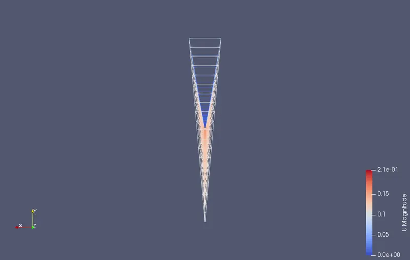
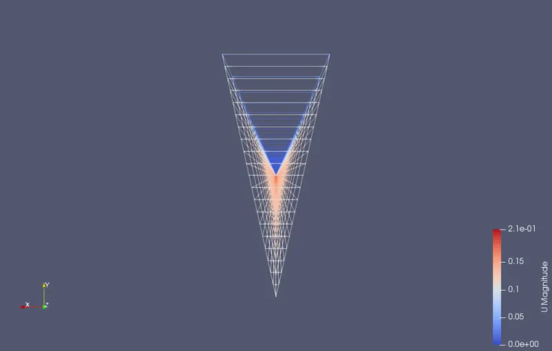
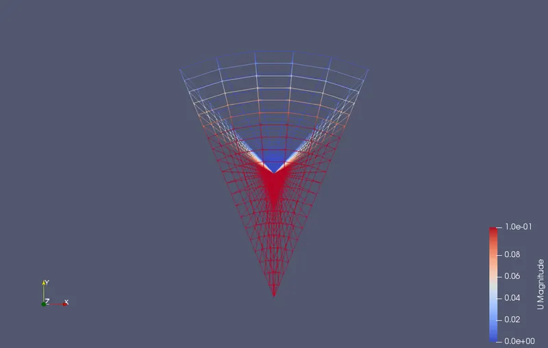
The meshed wedge is shown below,the meshing was successful without any errors
10 degree mesh
25 degree mesh
45 degree mesh
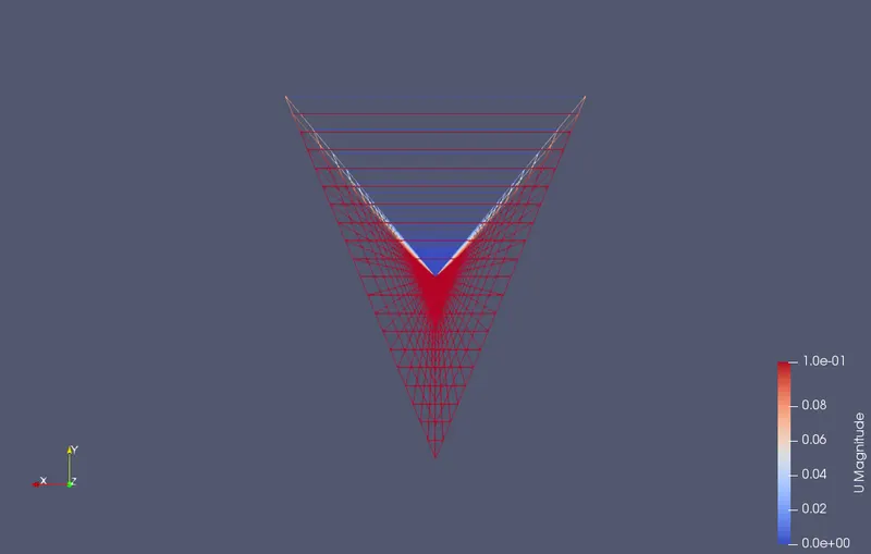
45 degree mesh with 5 cells along the y direction. taking this mesh drastically increases the computational time required to simulate the flow
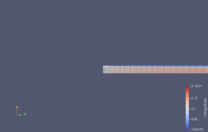
The velocity profile for fully developed flow :
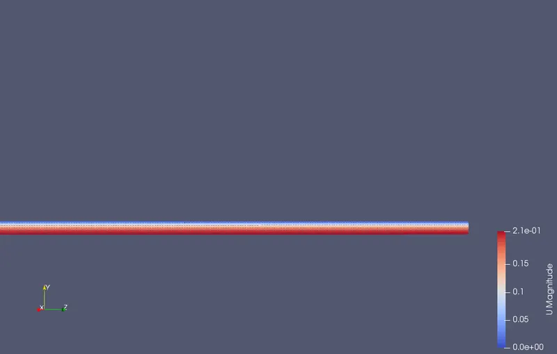
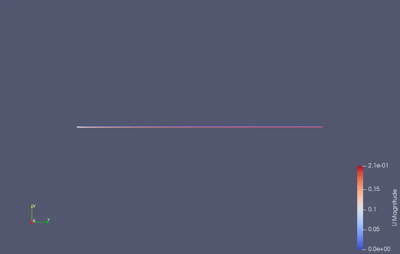
We can see how the flow develops and the values of velocity change. we can see the upper wall has a velocity of 0 (noslip boundary condition) we can also see how the velocity is the highest at the tip of the wedge which co-relates to the physics that describes the flow. Simulation results are visually very similar in both the wedge and symmetryPlane boundary condition. thus the images below are representative of how the simulation looks like for all cases.
At entry
at exit
full simulation
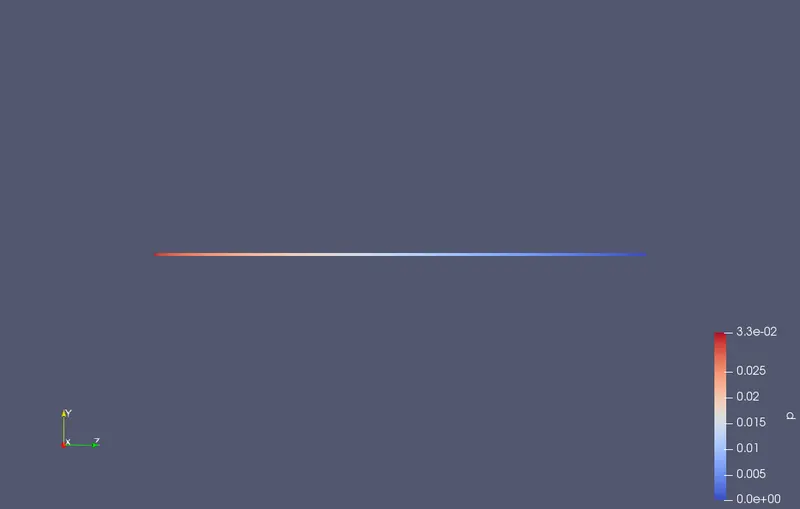
The pressure profile for fully developed flow
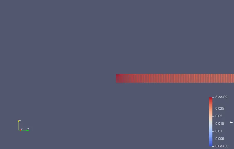
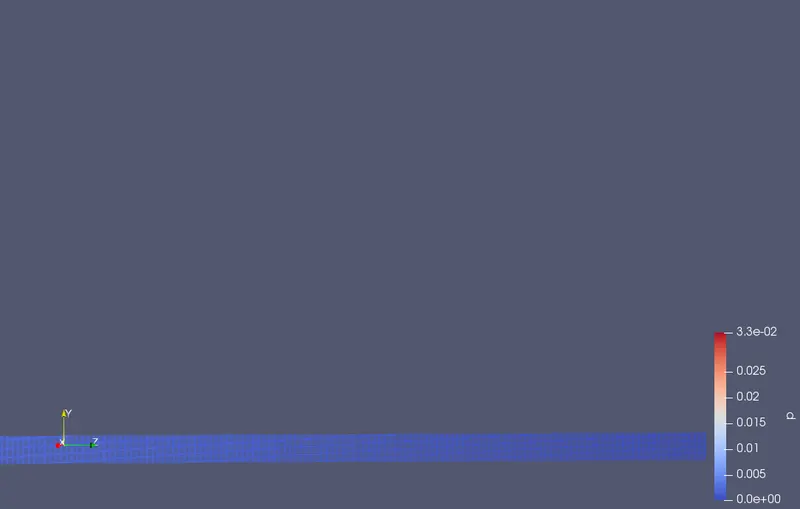
the simulation results for pressure at the entry, exit and overall view. we can see how the pressure changes throughout the pipe, being the highest at the entry and the lowest at the exist. the drop in pressure is called head loss or pressure drop.Simulation results are visually very similar in both the wedge and symmetryPlane boundary condition. thus the images below are representative of how the simulation looks like for all cases.
Velocity comparison
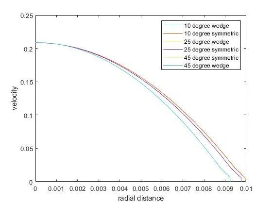
- we can see that as the wedge angle increases the accuracy decreases
- we can see that although we have used 2 different methods ie wedge and symmetryPlane the simulation results are identical thus the presence of only 3 visible curves in the above graph
- we can see that this above values resemble that described by the physics of the problem thus we can say that our simulation is successful
Shear Stress comparison
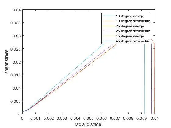
- We can see that as the wedge angle increases the value of shear stress increases
- We can see that although we have used 2 different methods ie: wedge and symmetryPlane. The simulation results are identical thus the presence of only 3 visible curves in the above graph
- We can see that this above values resemble that described by the physics of the problem thus we can say that our simulation is successful