1D Super-sonic nozzle flow simulation using Macormack Method (MATLAB)

AIM:

This project will simulate the isentropic flow through a quasi 1D subsonic-supersonic nozzle. Derive both the conservation and non-conservation forms of the governing equations and sovle them using the MacCormack's technique.

OBJECTIVE:

plot the following

1. Steady-state distribution of primitive variables inside the nozzle
2. Time-wise variation of the primitive variables
3. Variation of Mass flow rate distribution inside the nozzle at different time steps during the time-marching process
4. Comparison of Normalized mass flow rate distributions of both forms
5. perform the grid independence test.

THEORY:

MacCormac Technique:

In CFD macCormac technique is a widely used descritization technique for the numerical solution of hyperbolic partial differential equations.

The MacCormack method is a variation of the two-step Lax–Wendroff scheme but is much simpler in application. To illustrate the algorithm, consider the following first order hyperbolic equation

Predictor step: In the predictor step, a "provisional" value of at time level (denoted by ) is estimated as follows

The above equation is obtained by replacing the spatial and temporal derivatives in the previous first order hyperbolic equation using forward differences.

Corrector step: In the corrector step, the predicted value is corrected according to the equation

Note that the corrector step uses backward finite difference approximations for spatial derivative. The time-step used in the corrector step is in contrast to the used in the predictor step.

The application of MacCormack method to the above equation proceeds in two steps; a predictor step which is followed by a corrector step.In the code we have used forward difference in the predictor step and backward difference in the corrector step(The order of differencing can be reversed for the time step). The final solution is the average of the sum of the values from the predictor and corrector step.

1D supersonic nozzle:

We consider the steady, isentropic flow through a convergent-divergent nozzle as shown in the figure below. the flow comes from a reservoir where the pressure and temperature are denoted by p0 and T0 respectively.the cross-sectional area of the reservoir is very large, hence the velocity is very small. the flow expands isentroopically to supersonic speeds at the nozzle exit.

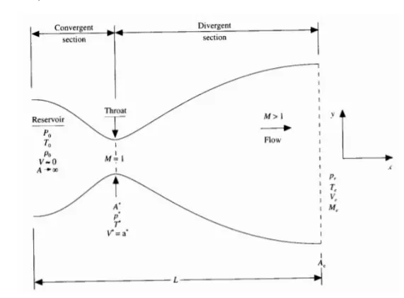
the nozzle consists of convergent, divergent and throat sections. the speed of the flow is less than the speed of sound in the convergent section, it is faster than the speed of sound at the divergent section and equal to the speed of sound at the throat ie mach number =1. The area of the nozzle changes as a function of the length along the x axis.

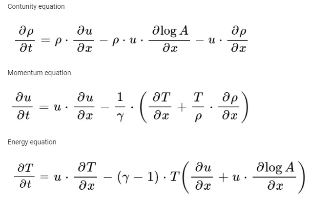
Governing Equation Of the Flow

1. Non-Conservative equations
   
2. Conservative Equations
   
   Continuity equation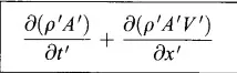
   
   
   Momentum equation
   
   
   Energy equation
   
   
   the above equation are in the non dimensionalised form, with the variables used as represented below.the formula's of the solution vector,state terms and the flux terms are as shown below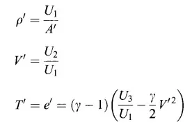
   
   
   
   
   
   
   
   
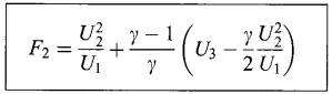
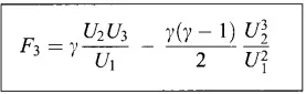
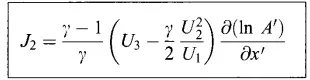
3. time step calculation
   
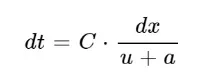
   c= courant number, 0.5 for the solution to be stable.
   dx= node size
   u= local velocity
   a=local speed of sound.

Initial and Boundary conditions

1. Non-Conservative method.
   
   rho=1-0.3146*x; %density
   temp= 1-0.2314*x; % temperature
   v=(0.1+1.09*x).*temp.^0.5;% velocity
   a=1 + 2.2*(x-1.5).^2; %area
   
   inlet conditions
   v(1)=2*v(2)-v(3);
   
   outlet conditions
   v(n)=2*v(n-1)-v(n-2);
   rho(n)=2*rho(n-1)-rho(n-2);
   temp(n)=2*temp(n-1)-temp(n-2);
   
   
   
2. Conservative method.
   
   
   
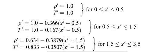
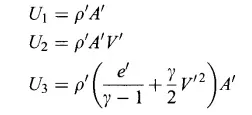
   %inlet
   u1(1)=a(1);
   u2(1)=2*u2(2)-u2(3);
   u3(1)=u1(1)*((temp_c(1)/(gamma-1)) + 0.7*(v_c(1)^2));
   %outlet
   u1(n)=2*u1(n-1)-u1(n-2);
   u2(n)=2*u2(n-1)-u2(n-2);
   u3(n)=2*u3(n-1)-u3(n-2);

CODE:

The following code was written on matlab. The simulation code is as shown below

clear all
close all
clc

nt=1400;
% calling non conservative function  
tic
[v,rho,temp,m,mach_no,p,rho_t,v_t,temp_t,p_t,mach_no_t,m_t,x]=nozzle_nonconservative();
non_conservative=toc;

%calling conservative function 
tic
[v_c,rho_c,temp_c,m_c,mach_no_c,p_c,rho_ct,v_ct,temp_ct,p_ct,mach_no_ct,m_ct]=nozzle_conservative();
conservative=toc;

%plotting conservative vs non conservative
%mass flow rate 
figure(3)
subplot(3,2,1)
plot(x,m);
hold on 
plot(x,m_c,'*');
%analytical solution is 0.579
a=0.579*ones(1,31);
plot(x,a,'-');
xlabel('non-dimensional flow throw the nozzle (x)');
ylabel('non-dimensional mass flow throw the nozzle (m)');
legend('non-conservative','conserative','analytical');
title('mass flow rate comparison');
grid on 

%variation of non dimentional flow parameters
%mach number
subplot(3,2,2)
plot(x,mach_no);
hold on 
plot(x,mach_no_c,'*');
xlabel('nozzle distace');
ylabel('mach number');
legend('non-conservative','conserative');
title('mach number comparison');
grid on 

%pressure
subplot(3,2,3)
plot(x,p);
hold on 
plot(x,p_c,'*');
xlabel('nozzle distace');
ylabel('presssure');
legend('non-conservative','conserative');
title('pressure comparison');
grid on 

%density
subplot(3,2,4)
plot(x,rho);
hold on 
plot(x,rho_c,'*');
xlabel('nozzle distace');
ylabel('density');
legend('non-conservative','conserative');
title('density comparison');
grid on 

%temperature
subplot(3,2,5)
plot(x,temp);
hold on 
plot(x,temp_c,'*');
xlabel('nozzle distace');
ylabel('temperature');
legend('non-conservative','conserative');
title('temperature comparison');
grid on 

%velocity
subplot(3,2,6)
plot(x,v);
hold on 
plot(x,v_c,'*');
xlabel('nozzle distace');
ylabel('velocity');
legend('non-conservative','conserative');
title('velocity comparison');
grid on 

% variation of flow at throat 
figure(4)
%plotting density 
subplot(4,1,1)
plot(1:nt,rho_t)
hold on 
plot(1:nt,rho_ct,'r')
ylabel('density');
legend('non-conservative','conserative');
title('density comparison at throat for various time step ');


%plotting temperature
subplot(4,1,2)
plot(1:nt,temp_t)
hold on 
plot(1:nt,temp_ct,'r')
ylabel('temperature');
legend('non-conservative','conserative');
title('temperature comparison at throat for various time step ');

%pressure
subplot(4,1,3)
plot(1:nt,p_t)
hold on 
plot(1:nt,p_ct,'r')
ylabel('pressure');
legend('non-conservative','conserative');
title('pressure comparison at throat for various time step ');

%mach number
subplot(4,1,4)
plot(1:nt,mach_no_t)
hold on 
plot(1:nt,mach_no_ct,'r')
ylabel('mach number');
legend('non-conservative','conserative');
title('mach number comparison at throat for various time step ');

The conservative function is as shown below

function [v_c,rho_c,temp_c,m_c,mach_no_c,p_c,rho_ct,v_ct,temp_ct,p_ct,mach_no_ct,m_ct]=nozzle_conservative()
%non conservative approach
%inputs
n=31;
x=linspace(0,3,n);
dx=x(2)-x(1);
l=[1:1400];
%calculating initial profiles 
%initialising density and temperature for conservative form.
for i=1:length(x)   
    if x(i)>=0 && x(i)<=0.5
        rho_c(i)=1;
        temp_c(i)=1;
    elseif x(i)>0.5 && x(i)<=1.5
        rho_c(i)= 1-0.366*(x(i)-0.5);
        temp_c(i)=1-0.167*(x(i)-0.5);
    elseif x(i)>1.5 && x(i)<=3
        rho_c(i)= 0.634-0.3879*(x(i)-1.5);
        temp_c(i)=0.833-0.3507*(x(i)-1.5);
    end
end
 

gamma =1.4;
a=1 + (2.2*((x-1.5).^2)); % nozzle area 
c=0.5; %cfl condition for stability
nt=1400; % no of time steps
throat=(n+1)/2;
v_c=0.59./(rho_c.*a);% velocity
for i=1:n
    dt_calc(i) = c.*(dx./(sqrt(temp_c(i))+v_c(i))); 
end
dt= min(dt_calc);
%dt = 0.0267;



%solution vector in terms of initial condition
u1= rho_c.*a;
u2= rho_c.*a.*v_c;
u3= rho_c.*((temp_c./(gamma-1))+(gamma./2)*(v_c.^2))    .*a;

  

 for k=1:1400
   % storing the old values of u1, u2 and u3 
    u1_old=u1;
    u2_old=u2;
    u3_old=u3;
    %flux variables for predictor step 
    f1=u2;
    f2=((u2.^2)./u1) + ((gamma-1)./gamma).*(u3 - (gamma/2).*((u2.^2)./u1));  
    f3=((gamma.*u2.*u3)./u1) - ((gamma.*(gamma-1))./2).*((u2.^3)./(u1.^2));




% %     predictor method 
    for j=2:n-1
        
      %  calculating the source term j2 
        j2(j)=(1/gamma)*rho_c(j)*temp_c(j)*((a(j+1)-a(j))/dx);
        
       % continuity equation
        du1dt_p(j) = -(f1(j+1)-f1(j))/dx;
       % momentum equation 
        du2dt_p(j) = -((f2(j+1)-f2(j))/dx)+j2(j);
       % energy equation 
        du3dt_p(j) = -(f3(j+1)-f3(j))/dx;
        
        %solution update 
        u1(j)=u1_old(j) + (du1dt_p(j)*dt);
        u2(j)=u2_old(j) + (du2dt_p(j)*dt);
        u3(j)=u3_old(j) + (du3dt_p(j)*dt);
    
       % decode the predicted values of primitive variables using u1 u2 u3 
%         rho_c(j)=u1(j)/a(j);
%         temp_c(j)= (gamma-1)*((u3(j)/u1(j))-(gamma/2)*(u2(j)/u1(j))^2);
%         v_c(j)=u2(j)/u1(j);
%         p_c(j)=rho_c(j)*temp_c(j);
    end
    
   % decode the predicted values of primitive variables using u1 u2 u3 
        rho_c= u1./a;
        temp_c= (gamma-1)*((u3./u1)-(gamma/2)*(u2.^2./u1.^2));
        v_c= u2./u1;
        p_c=rho_c.*temp_c;
        
    %flux variables for corrector step (check)
    f1=u2;
    f2=((u2.^2)./u1) + ((gamma-1)/gamma).*(u3 - (gamma/2).*((u2.^2)./u1));  
    f3=((gamma.*u2.*u3)./u1) - ((gamma*(gamma-1))/2).*((u2.^3)./(u1.^2));
    
     %corrector method 
    for j=2:n-1
        
        % calculating the source term j2- updated 
        j2(j)=(1/gamma)*rho_c(j)*temp_c(j)*((a(j)-a(j-1))/dx);
        
        %continuity equation
        du1dt_c(j) = -(f1(j)-f1(j-1))/dx;
        %momentum equation 
        du2dt_c(j) = -((f2(j)-f2(j-1))/dx)+j2(j);
        %energy equation 
        du3dt_c(j) = -(f3(j)-f3(j-1))/dx;
    end
    
      %computing the average time derivative 
    du1dt= 0.5.*(du1dt_p + du1dt_c);
    du2dt= 0.5.*(du2dt_p + du2dt_c);
    du3dt= 0.5.*(du3dt_p + du3dt_c);
    
    %calculating the residual 
    du1dt_t(k)= du1dt(throat);
    du2dt_t(k)= du2dt(throat);
    du3dt_t(k)= du3dt(throat);
    
    %final solution update 
     for j=2:n-1
        u1(j)= u1_old(j) + (du1dt(j).*dt);
        u2(j)= u2_old(j) + (du2dt(j).*dt);
        u3(j)= u3_old(j) + (du3dt(j).*dt);
     end
     
     %applying boundary conditions
     %inlet 
     u1(1)=a(1);
     u2(1)=2*u2(2)-u2(3);
     v_c(1) = u2(1)/u1(1);
     u3(1)=u1(1)*((temp_c(1)/(gamma-1)) + 0.7*(v_c(1)^2));
     
     %outlet
     u1(n)=2*u1(n-1)-u1(n-2);
     u2(n)=2*u2(n-1)-u2(n-2);
     u3(n)=2*u3(n-1)-u3(n-2);
     
     % decode the predicted values of primitive variables using u1 u2 u3 
    rho_c= u1./a;
    temp_c= (gamma-1)*((u3./u1)-(gamma/2)*(u2.^2./u1.^2));
    v_c= u2./u1;
    p_c=rho_c.*temp_c;
     %mass flow rate m
     m_c=rho_c.*a.*v_c;
     %pressure ratio 
     p_c=rho_c.*temp_c;
     %mach no
     mach_no_c = v_c./sqrt(temp_c);

     %VALUEs at throat 
     rho_ct(k)=rho_c(throat);
     v_ct(k)=v_c(throat);
     temp_ct(k)=temp_c(throat);
     p_ct(k)=p_c(throat);
     mach_no_ct(k)=  mach_no_c(throat);
     m_ct(k)=m_c(throat);
     
      %plotting mass flow rate at different time steps 
    figure(2);
    if k==50
        plot(x,m_c,'color','b','linewidth',1.5);
        hold on 
    elseif k == 100
        plot(x,m_c,'color','g','linewidth',1.5);
        hold on 
    elseif k == 150
        plot(x,m_c,'color','y','linewidth',1.5);
        hold on 
    elseif k == 200
        plot(x,m_c,'color','black','linewidth',1.5);
        hold on 
    elseif k == 500
        plot(x,m_c,'color','cyan','linewidth',1.5);
        hold on 
    elseif k == 700
        plot(x,m_c,'color','r','linewidth',1.5);
        hold on 
    elseif k == 1400
        plot(x,m_c,'color','m','linewidth',1.5);
        grid on    
    end
end
hold off
% 'Name','Mass flow rate at diff time step'
xlabel('non-dimensional flow throw the nozzle (x)');
ylabel('non-dimensional mass flow throw the nozzle (m)');
legend({'50 time steps','100 time steps','150 time steps','200 time steps','500 time steps','700 time steps','1400 time steps'});

figure(6)
semilogy(l,du1dt_t,'r');
hold on
semilogy(l,du2dt_t,'b');
semilogy(l,du3dt_t,'g');
xlabel('number of time steps ');
ylabel('values of residualat throat');
legend('du1dt','du2dt','du3dt');



end

   

The non-conservative function is as shown below

function [v,rho,temp,m,mach_no,p,rho_t,v_t,temp_t,p_t,mach_no_t,m_t,x]=nozzle_nonconservative()
%non conservative approach
%inputs
n=31;
x=linspace(0,3,n);
dx=x(2)-x(1);

%calculating initial profiles 
rho=1-0.3146*x; %density 
temp= 1-0.2314*x; % temperature
v=(0.1+1.09*x).*temp.^0.5;% velocity
gamma =1.4;

a=1 + 2.2*(x-1.5).^2;
c=0.5; %cfl condition for stability
nt=1400;
l=[1:1400];
throat=(n+1)/2;
dt=min(c.*(dx./(sqrt(temp)+v)));
% dt=0.02;
%outer time loop 
for k=1:nt
    
    rho_old=rho;
    v_old=v;
    temp_old=temp;
    %predictor method 
    for j=2:n-1
       %drho_dt_p = -rho(j)*(v(j+1)-v(j))/dx - rho(j)*v(j)*(log(a(j+1))-log(a(j)))/dx-v(j)*(rho(j).....)
        dvdx=(v(j+1)-v(j))/dx;
        drhodx=(rho(j+1)-rho(j))/dx;
        dtdx=(temp(j+1)-temp(j))/dx;
        dlogadx=(log(a(j+1))-log(a(j)))/dx;
        %continuity equation
        drhodt_p(j) = -rho(j)*dvdx -rho(j)*v(j)*dlogadx-v(j)*drhodx;
        
        %momentum equation 
        dvdt_p(j) =-v(j)*dvdx -(1/gamma)*(dtdx+(temp(j)/rho(j))*drhodx);
        
        %energy equation
        dtdt_p(j)=-v(j)*dtdx-(gamma-1)*temp(j)*(dvdx+v(j)*dlogadx);
        
        %solution update
        rho(j)=rho(j)+drhodt_p(j)*dt;
        v(j)=v(j)+dvdt_p(j)*dt  ;
        temp(j)=temp(j)+dtdt_p(j)*dt;
        
    end
    
        %corrector method 
    for j=2:n-1
       %drho_dt_p = -rho(j)*(v(j+1)-v(j))/dx - rho(j)*v(j)*(log(a(j+1))-log(a(j)))/dx-v(j)*(rho(j).....)
        dvdx=(v(j)-v(j-1))/dx;
        drhodx=(rho(j)-rho(j-1))/dx;
        dtdx=(temp(j)-temp(j-1))/dx;
        dlogadx=(log(a(j))-log(a(j-1)))/dx;
        %continuity equation
        drhodt_c(j) = -rho(j)*dvdx -rho(j)*v(j)*dlogadx-v(j)*drhodx;
        
        %momentum equation 
        dvdt_c(j) =-v(j)*dvdx -(1/gamma)*(dtdx+(temp(j)/rho(j))*drhodx);
        
        %energy equation
        dtdt_c(j)=-v(j)*dtdx-(gamma-1)*temp(j)*(dvdx+v(j)*dlogadx);
        
%         %solution update
%         rho(j)=rho(j)+drhodt_c(j)*dt;
%         v(j)=v(j)+dvdt_c(j)*dt  ;
%         temp(j)=temp(j)+dtdt_c(j)*dt;
    end
    %computing the average time derivative 
    dvdt= 0.5*(dvdt_p + dvdt_c);
    drhodt= 0.5*(drhodt_p + drhodt_c);
    dtdt= 0.5*(dtdt_p + dtdt_c);
    
    %calculating residual 
    dvdt_t(k)=abs(dvdt(throat));
    drhodt_t(k)=abs(drhodt(throat));
    dtdt_t(k)=abs(dtdt(throat));
   
    %final solution update
    
    for i=2:n-1
        v(i)=v_old(i)+dvdt(i)*dt;
        rho(i)=rho_old(i)+drhodt(i)*dt;
        temp(i)=temp_old(i)+dtdt(i)*dt;
    end
    %applying boundary conditions
    %inlet
    v(1)=2*v(2)-v(3);
    
    %outlet
    v(n)=2*v(n-1)-v(n-2);
    rho(n)=2*rho(n-1)-rho(n-2);
    temp(n)=2*temp(n-1)-temp(n-2);
    
    %mass flow rate m
    m=rho.*a.*v;
    %pressure ratio 
    p=rho.*temp;
    %mach no
    mach_no = v./sqrt(temp);
    
    %VALUEs at throat 
    rho_t(k)=rho(throat);
    v_t(k)=v(throat);
    temp_t(k)=temp(throat);
    p_t(k)=p(throat);
    mach_no_t(k)=  mach_no(throat);
    m_t(k)=m(throat);
    
    %plotting mass flow rate at different time steps 
    figure(1);
    if k==50
        plot(x,m,'color','b','linewidth',1.5);
        hold on 
    elseif k == 100
        plot(x,m,'color','g','linewidth',1.5);
        hold on 
    elseif k == 150
        plot(x,m,'color','y','linewidth',1.5);
        hold on 
    elseif k == 200
        plot(x,m,'color','black','linewidth',1.5);
        hold on 
    elseif k == 500
        plot(x,m,'color','cyan','linewidth',1.5);
        hold on 
    elseif k == 700
        plot(x,m,'color','r','linewidth',1.5);
        hold on 
    elseif k == 1400
        plot(x,m,'color','m','linewidth',1.5);
        grid on    
    end
end
hold off
% 'Name','Mass flow rate at diff time step'
xlabel('non-dimensional flow throw the nozzle (x)');
ylabel('non-dimensional mass flow throw the nozzle (m)');
legend({'50 time steps','100 time steps','150 time steps','200 time steps','500 time steps','700 time steps','1400 time steps'});

figure(5)
semilogy(l,dvdt_t,'r');
hold on
semilogy(l,drhodt_t,'b');
semilogy(l,dtdt_t,'g');
xlabel('number of time steps ');
ylabel('values of residualat throat');
legend('dvdt','drhodt','dTdt');


end

OUTPUT AND CONCLUSION:

The output graphs are shown below

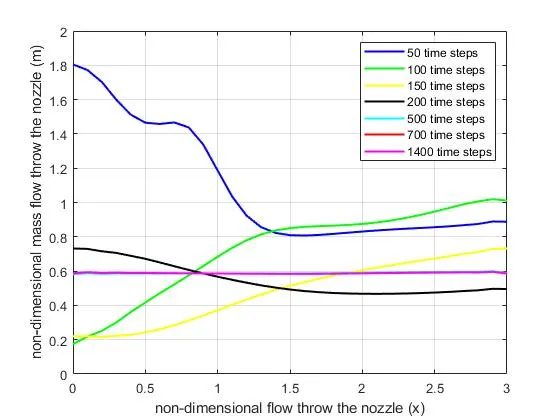
nonconservative mass flow wrt time step

7 different mass flow rate values are plotted at various time steps.We can see that in the initial timesteps the massflow rate varies from the convergent stage to the divergent stage, but after achieving steady state(around 700 iterations ) the variation is minimal.

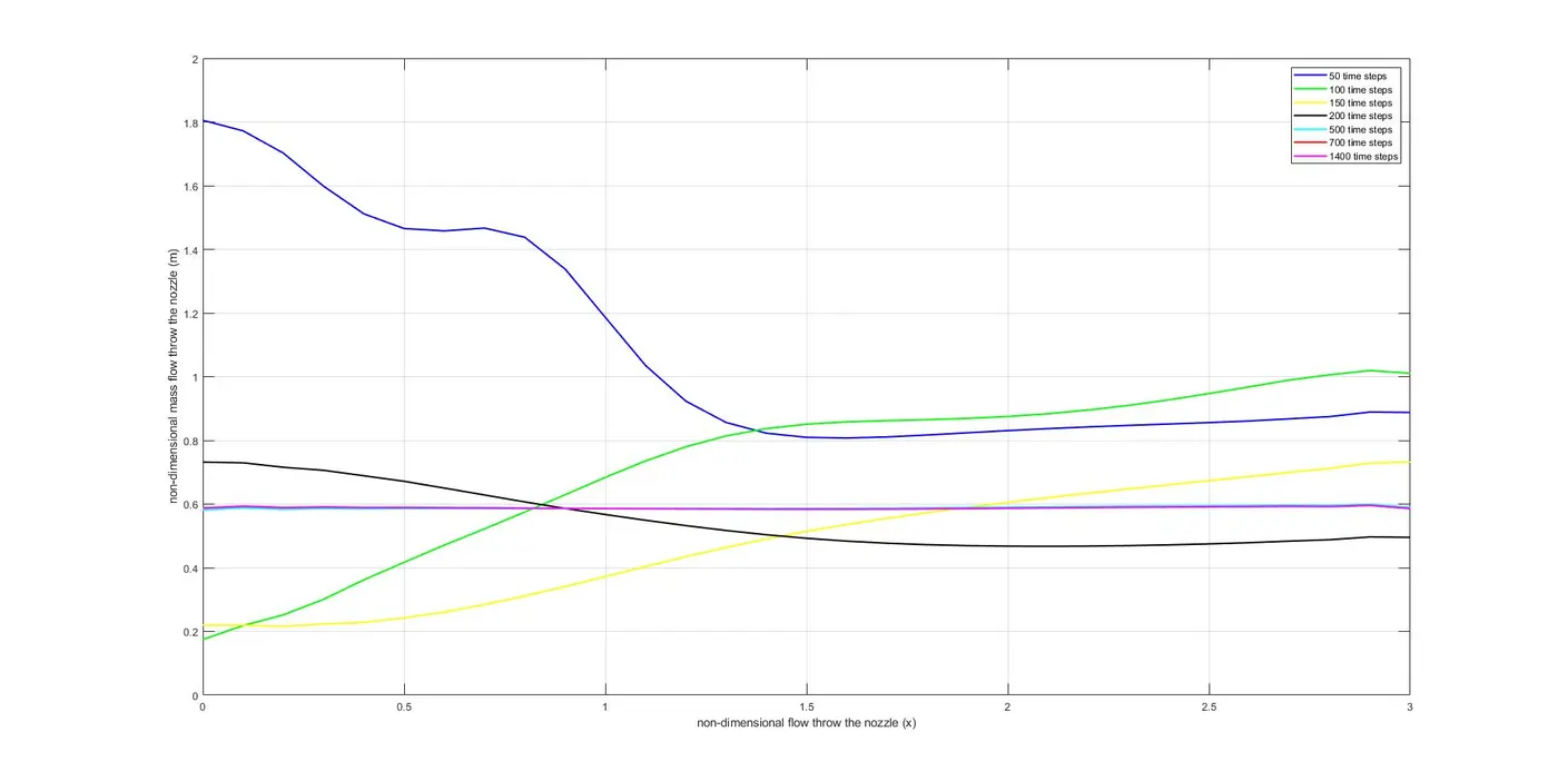
conservative wrt time step

7 different mass flow rate values are plotted at various time steps.We can see that in the initial timesteps the massflow rate varies from the convergent stage to the divergent stage,and the values of mass flow rate is very high but after 200 iterations the values approach steady state. after achieving steady state(around 700 iterations ) the variation is minimal.

Comparing the mass flow rate between conservative and non conservative we can say

1. conservative form produces better results with lesser diviation
2. conservative form produces better results due to the presence of the flux terms

Conservative vs Non-Conservative

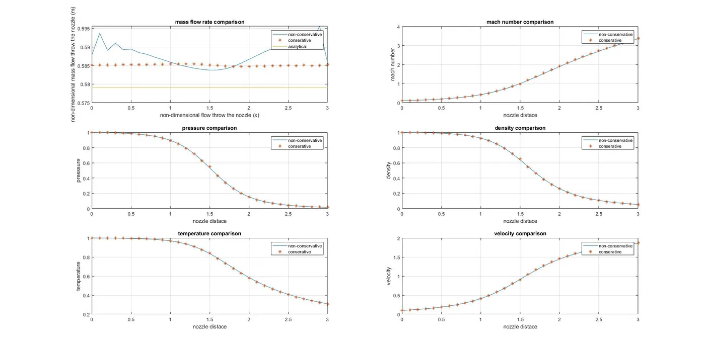
we can see from above

1. mass flow rate in non conservative method has relatively more variation as compared to conservative method
2. both mass flow rate of conservative and non conservative are not equal to the analytical plot
3. the primitive variable are almost identical.

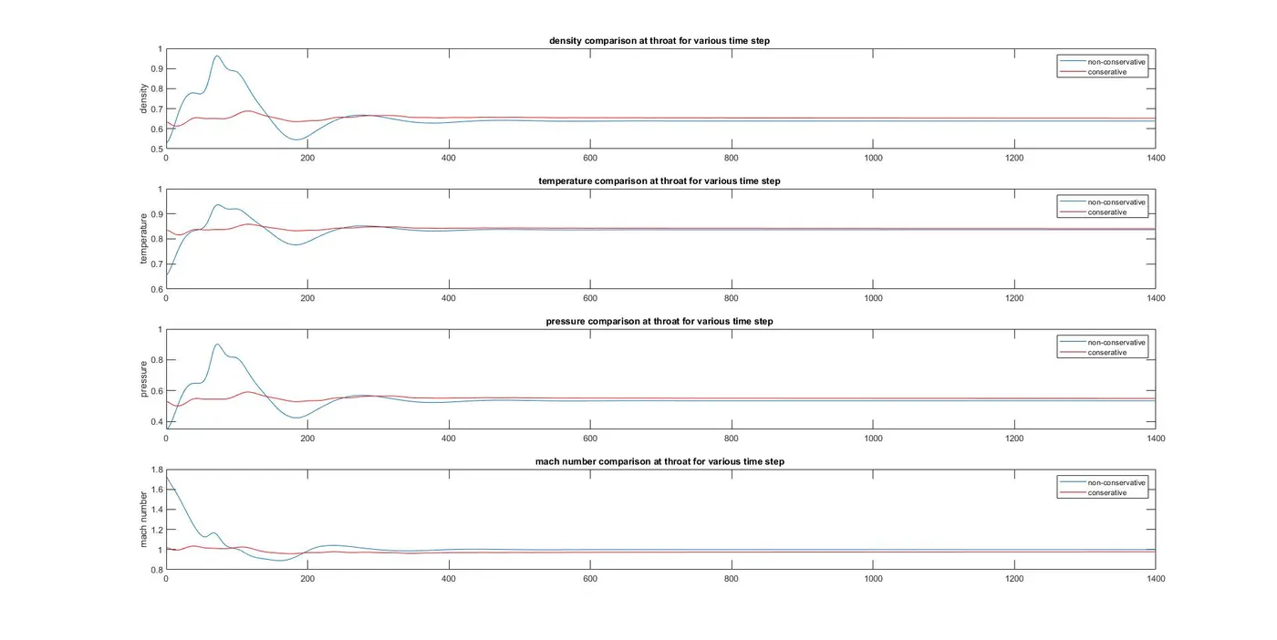
we can see from above

1. the graph is plotted for the variation of values at the throat for various time steps
2. the values approach stability with more time steps
3. there are more oscillations in the 0-200 range and then they gradually reduce
4. non-conservative form tends to fluctuate more
5. a minimum of 600 iterations need to be provided for convergence.
6. the conservative method tends to converge faster

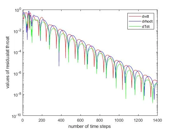
The graph of the residuals

nonconservative form

conservative form

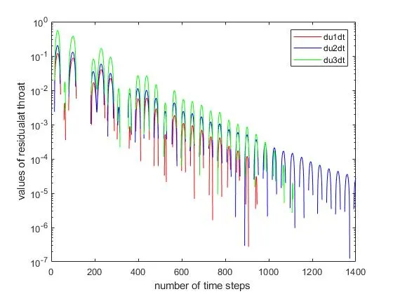
from the above graphs we can see that in both cases as the time step increases the size of the residual gets smaller, this shows that convergence is being reached. Since all the residuals are under 10^-5 we can say that we have attained convergence.we can also see that the residuals of the non conservative form is lower than that of the conservative form, thus we can say that the non conservative form can reach steady state faster than the conservative method.

GRID DEPENDENCE TEST:

To conduct the grid dependence test we need to change the number of grid points we are taking

	Density ratio	Temperature ratio	Pressure ratio	Mach number
Exact analytical solution	0.634	0.833	0.528	1
non-conservational form (n=31)	0.6387	0.8365	0.5342	0.9994
conservational form (n=31)	0.6524	0.8410	0.5487	0.9780
non-conservational form (n=61)	0.6377	0.8354	0.5327	0.9998
conservational form (n=61)	0.6391	0.8355	0.5340	0.9979

The values are taken at the throat

We can see that as we change the number of grid point the values get closer to the analytical solution, but only marginally.

Due to the increase in the number of grid points the run time increases significantly.

we can also wee that the nonconservational form with 61 grid points results in the solution closest to the analytical solution.

PS: the conclusions are mentioned with the graphs.