Project 2 - Rankine cycle Simulator

AIM:

To understand the Rankine Cycle and to simulate it using MATLAB

Objective:

1. To accept in initial conditions from the user.
2. To calculate the state variables at each point
3. To calculate the net work output, SSC, Back work ratio
4. To plot the T-S and H-S graphs.

THEORY:

In general, the Rankine cycle is an idealized thermodynamic cycle of a constant pressure heat engine that converts part of heat into mechanical work. In this cycle the heat is supplied externally to a closed loop, which usually uses water (in a liquid and vapor phase) as the working fluid. The working fluid in the Rankine cycle undergoes the phase change from a liquid to vapor phase and vice versa.

While many substances could be used as the working fluid in the Rankine cycle (inorganic or even organic),water is usually the fluid of choice due to its favorable properties, such as its non-toxic and unreactive chemistry, abundance, and low cost, as well as its thermodynamic properties. For example, water has the highest specific heat of any common substance – 4.19 kJ/kg K. Moreover it has very high heat of vaporisation, which makes it an effective coolant and medium in thermal power plants and other energy industry. In case of the Rankine cycle, the Ideal Gas Law almost cannot be used (steam do not follow pV=nRT), therefore all important parameters of water and steam are tabulated in so called “Steam Tables“.

CODE:

This code was done on MATLAB. explanation of the code is done through the comments in the code. XSteam function was used to get the steam table values of water, used in various states in the rankine cycle

%ideal rankine cycle simulator
%this process is entirely reversible 
%state 1 - out of the boiler (saturated vapour)
%state 2 - out of turbine
%state 3 - out of condenser (saturated liquid)
%state 4 - out of the pump.
%qb- heat into boiler 
%wt- work from turbine 
%qc- heat transfer out of condenser 
%wp- work into pump
%p1=p4>> p2=p3 
%w_net=w_turb-w_pump
%w_turb=h1-h2; kJ/kg
%w_pump= (p_1 -p_3)/10;
%efficiency= w_net/qb= w_net/h1-h4
%back_work_ratio= w_pump/w_turb
% need temp,pressure, enthalpy and entropy for each state 



clear all 
close all 
clc
disp('Rankine Cycle Simulator ');
disp('1-2 Isentropic expansion in the turbine ');
disp('2-3 Const pressure heat rejection in the condenser  ');
disp('3-4 Isentropic compression in the pump ');
disp('4-1 constant pressure heat adiition in the boiler ');
fprintf('\n \n');
% taking user defined input;
t_1=input('enter turbine inlet temperature(in celcius):'); % turbine inlet temp
p_1=input('enter turbine inlet pressure(in bar):'); % boiler pressure 
p_2= input('enter turbine outlet pressure(in bar):'); %condenser pressure 

t=XSteam('Tsat_p',p_1);
if t_1>=t;  % to check if the temp given is less than the saturation temp

    p_4=p_1;
    p_3=p_2;
    h1=XSteam('h_pT',p_1,t_1); % calling function to accept steam table data 
    s1=XSteam('s_pT',p_1,t_1);
    s2=s1;
    % s2=Sf +x*Sfg; x- dryness fraction 
    sf2=XSteam('sL_p',p_2);
    sg2=XSteam('sV_p',p_2);
    hf2=XSteam('hL_p',p_2);
    hg2=XSteam('hV_p',p_2);
    x2=((s2-sf2)/(sg2-sf2));
    h2 = hf2+(x2*(hg2-hf2));
    t_3=XSteam('Tsat_p',p_3);
    t_2=t_3;
    h3=hf2;
    s3=sf2;
    v3=XSteam('vL_p',p_2);
    h4=h3+(v3*(p_4-p_3))*100; % to convert to KJ
    s4=s3;
    
    % to calculate T4
    cp4=XSteam('Cp_ps',p_4,s4);
    cv4=XSteam('Cv_ps',p_4,s4);
    q=cp4/cv4;
    w=(q-1)/q; 
    t_4=t_3*((p_4/p_3)^w);
    
    % calculating the work and other quantities  
    w_turb=h1-h2; % work is in kJ/kg
    w_pump= h4-h3;
    w_net=w_turb-w_pump;
    back_work_ratio= w_pump/w_turb; % no units as it is a ratio
    ssc=3600/w_net;
    qb=h1-h4;
    qc=h2-h3;
    efficiency= (1-(qc/qb))*100; % percentage 
    % for process 4-1, isobaric
    t_5= XSteam('Tsat_p',p_1);
    s5=XSteam('sL_p',p_1);
    s6=XSteam('sV_p',p_1);
    % displaying info 
    fprintf('\n \n RESULTS \n ');
    fprintf('At state point 1:\n P1 is :%4.2f Bar \n T1 is:%4.2f degree celcius\n H1 is:%4.2f KJ/kg\n S1 is :%4.2f KJ/kgK \n \n',p_1,t_1,h1,s1);
    fprintf('At state point 2:\n P2 is :%4.2f Bar \n T2 is:%4.2f degree celcius\n H2 is:%4.2f KJ/kg\n S2 is :%4.2f KJ/kgK \n \n',p_2,t_2,h2,s2);
    fprintf('At state point 3:\n P3 is :%4.2f Bar \n T3 is:%4.2f degree celcius\n H3 is:%4.2f KJ/kg\n S3 is :%4.2f KJ/kgK \n \n',p_3,t_3,h3,s3);
    fprintf('At state point 4:\n P4 is :%4.2f Bar \n T4 is:%4.2f degree celcius\n H4 is:%4.2f KJ/kg\n S4 is :%4.2f KJ/kgK \n \n',p_4,t_4,h4,s4);
    fprintf(' Turbine work : %4.2f kJ/kg \n Pump work is :%4.2f kJ/kg \n Net work is :%4.2f kJ/kg \n Efficiency is : %4.2f percent \n Back work ratio : %4.5f \n SSC: %4.2fkg/kWh\n \n ',w_turb,w_pump,w_net,efficiency,back_work_ratio,ssc );

    % for the water vapour line 
    temp=linspace(1,400,400);
    for i=1:length(temp)
        a1(i)=XSteam('sL_t',temp(i));
        a2(i)=XSteam('sV_t',temp(i));
        a3(i)=XSteam('hL_t',temp(i));
        a4(i)=XSteam('hL_t',temp(i));

    end
    % plotting 
    subplot (1,2,1)
    plot([s1 s2 s3 s4 s5 s6 s1],[t_1 t_2 t_3 t_4 t_5 t_5 t_1],'linewidth',2,'marker','*','markersize',4);
    hold on 
    plot(a1,temp,'color','r');
    plot(a2,temp,'color','r');
    axis([0 10 0 700 ]);
    text(s1,t_1,'1','FontSize',10);
    text(s2,t_2,'2','FontSize',10);
    text(s3,t_3,'3','FontSize',10);
    text(s4,t_4,'4','FontSize',10);
    xlabel('S-entropy');
    ylabel('T- temperature');
    subplot(1,2,2)
    plot([s1 s2 s3 s4 s1],[h1 h2 h3 h4 h1],'linewidth',2,'marker','*','markersize',4);
    hold on 
    plot(a1,a3,'color','r');
    plot(a2,a4,'color','r');
    axis([0 10 0 4000 ]);
    text(s1,h1,'1','FontSize',10);
    text(s2,h2,'2','FontSize',10);
    text(s3,h3,'3','FontSize',10);
    text(s4,h4,'4','FontSize',10);
    xlabel('S - entropy');
    ylabel('H - enthalpy');
    
else
    fprintf('entered temperature is less than saturation temperature ')
end

    

ERRORS ENCOUNTERED :

• Basic synatx errors were encountered, these were shortly corrected
• Logic errors based on the rankine cycle, these were corrected and the cycle throughly understood

OUTPUT:

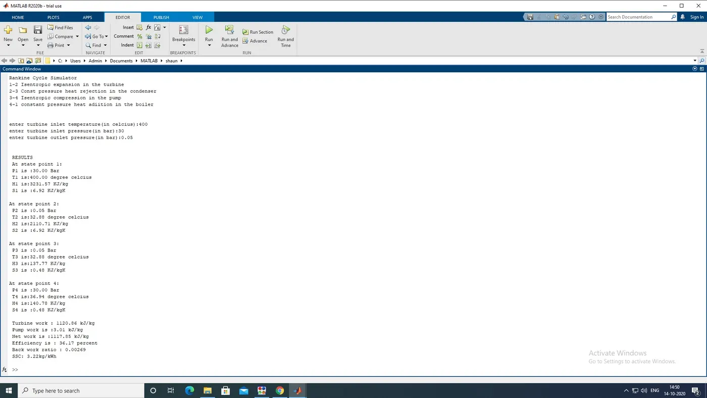
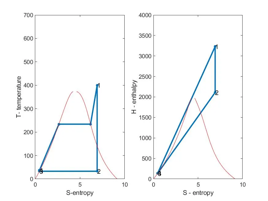
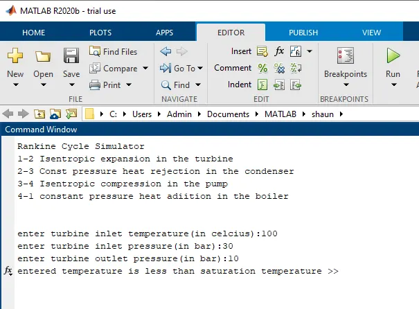
If the temperature inputed is less than the saturation temperature then the following output would be displayed.

CONCLUSION:

The rankine cycle was thoroughly understood and the calculations were written into the code, thus creating this simulation.