Simulating Combustion of Natural Gas. (ANSYS FLUENT)
AIM: To perform a 2D axisymmetric Combustion simulation With the given combustor model.
OBJECTIVES:
- plot the variation of the mass fraction of the different species’ in the simulation using line probes at different locations of the combustor. We need to plot for CO2, H2O, CH4, N2, O2, NOx emissions & Soot formation.
- Add the water content in the fuel from 5% to 30% by mole and observe the effect of it on the results. It is necessary to provide line plots and contours to prove your claim.
THEORY:
The value of slope coefficient increased on average within the range of 3.8% up to 8% per decade, which corresponds to the decrease in the number of heating hours of 22-139h during the heating season (depending on the combination of weather and renovation scenarios considered). On the other hand, function intercept increased by 7.8-12.7% per decade (depending on the coupled scenarios). The values suggested could be used to modify the function parameters for the scenarios considered, and Therefore, a drastic reduction in emissions is mandatory, demanding a deeper understanding of the formation process, which is still an open issue in combustion chemistry research.
In the past years, strategies for the reduction in soot emissions relied mainly on correlations, experience and trial and-error attempts. The increasing diffusion of CFD is allowing to analyze and optimize combustion devices with sufficient confidence. However, the uncertainty increases significantly when soot is concerned: the complexity of the gas-phase chemistry and the numerous mechanisms involved in the soot formation process, which are strongly coupled with mixing and radiative heat transfer and depend on soot volume fraction itself, make the prediction of soot emissions still a challenging task, leading to large errors in exhaust concentration even with small mispredictions in the formation rates.
Large IC engines such as ship engines spray water into the combustion chamber to reduce the mass fraction of pollutants such as NOX and soot.
CASE SETUP:
GEOMETRY:
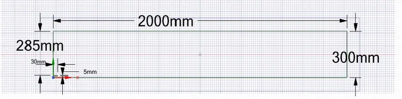
Open space claim and create the geometry as shown in the image below, the CH4 inlet is much smaller as compared to the air inlet.
MESHING:
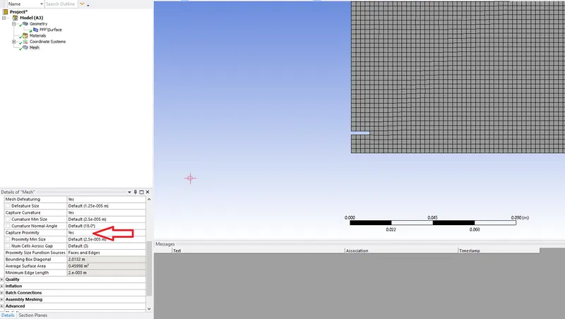
In the meshing interface, we need to give the names to the required selections. we need to enable the capture proximity option to get the best mesh. Images from the meshing interface are shown below.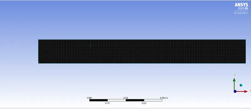
FLUENT:
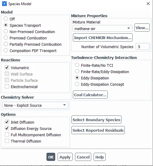
The general model setup was done as shown below 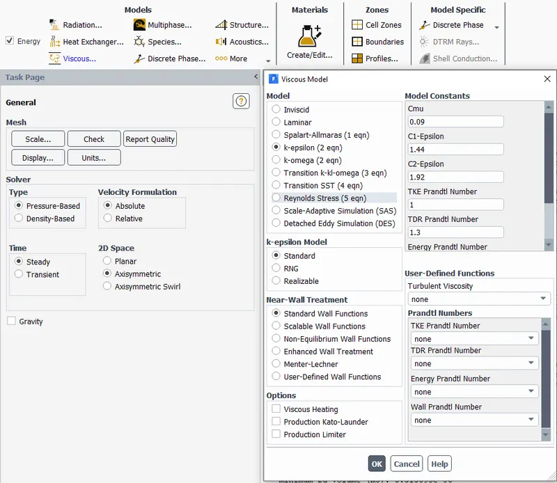
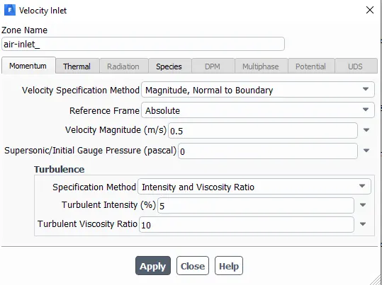
The velocity at the inlet for the air was set up as follows.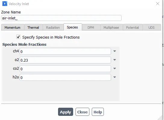
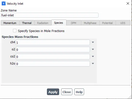
The velocity at the inlet for the fuel was set up as follows.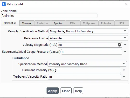
The Nox model was set up as 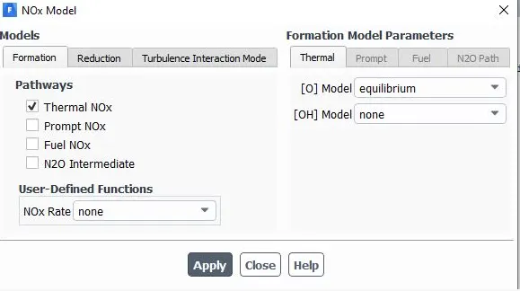
The soot model was setup as 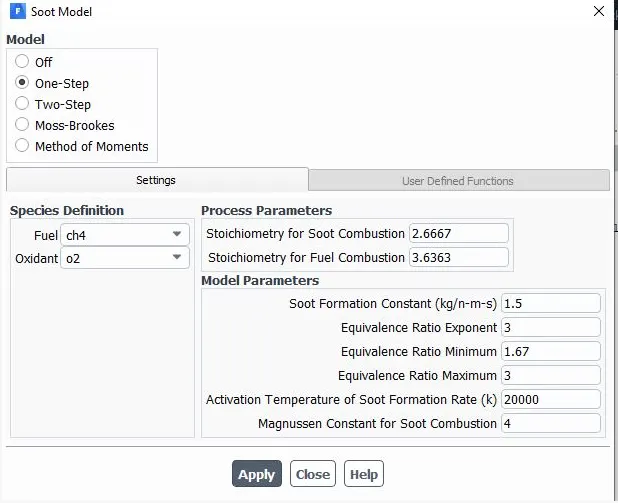
The simulation was thus setup and run.
SIMULATION RESULTS :
PART 1:plot the variation of the mass fraction of the different species’ in the simulation using line probes at different locations of the combustor as shown in Fig. You need to plot for CO2, H2O, CH4, N2, O2, NOx emissions & Soot formation.
This simulation is carried out without adding any water to the combustion (mass fraction of CH4 =1). This will provide us with baseline values for the next case.
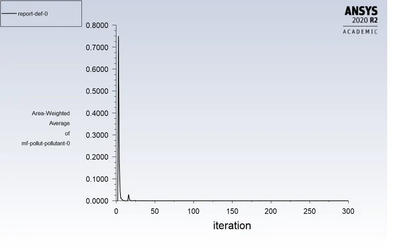
The first image is of the residuals, this tells us that the error has not grown and the simulation was run successfully 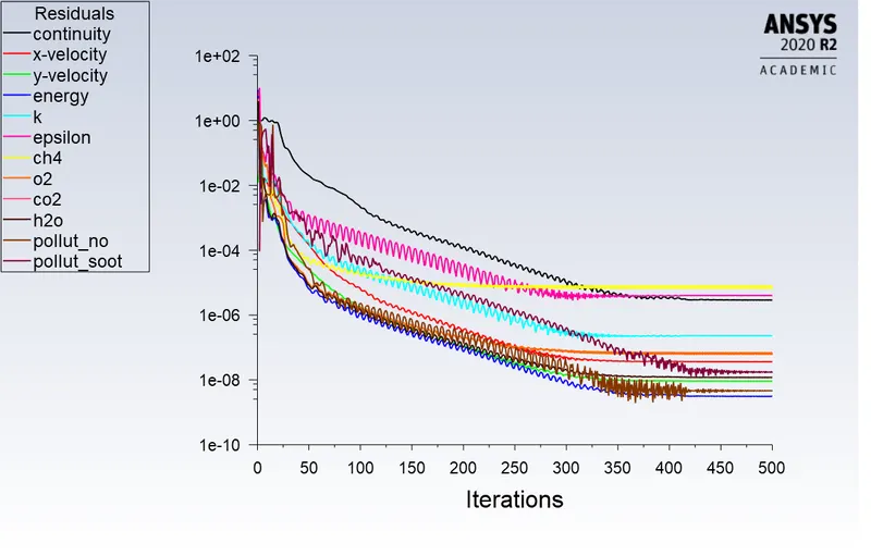
Using line probes we can measure the mass fraction of the quantity of interest (the location of the probe is mentioned in the legend of each image).
The plot of O2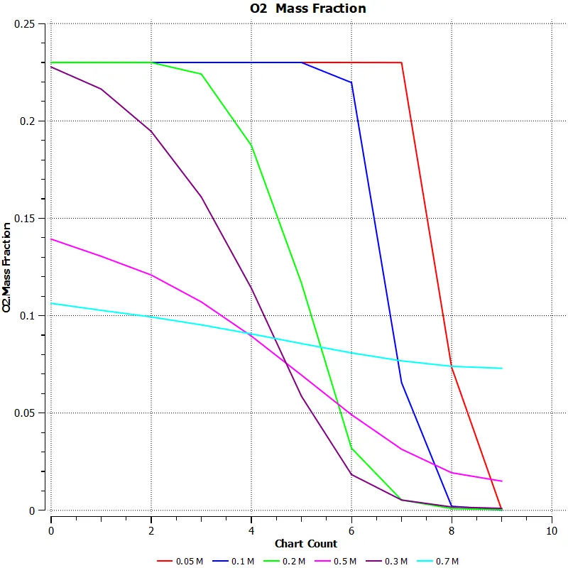
The plot for CH4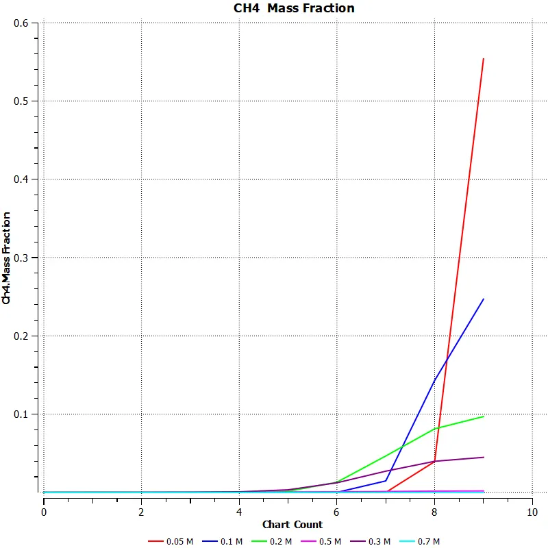
The plot for Co2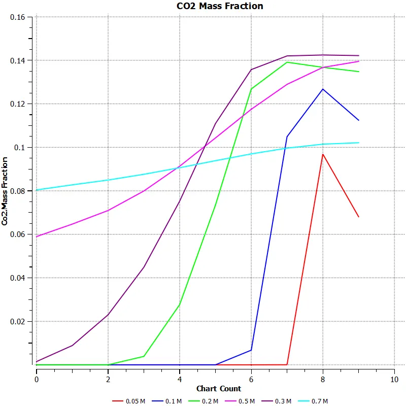
The plot for H2O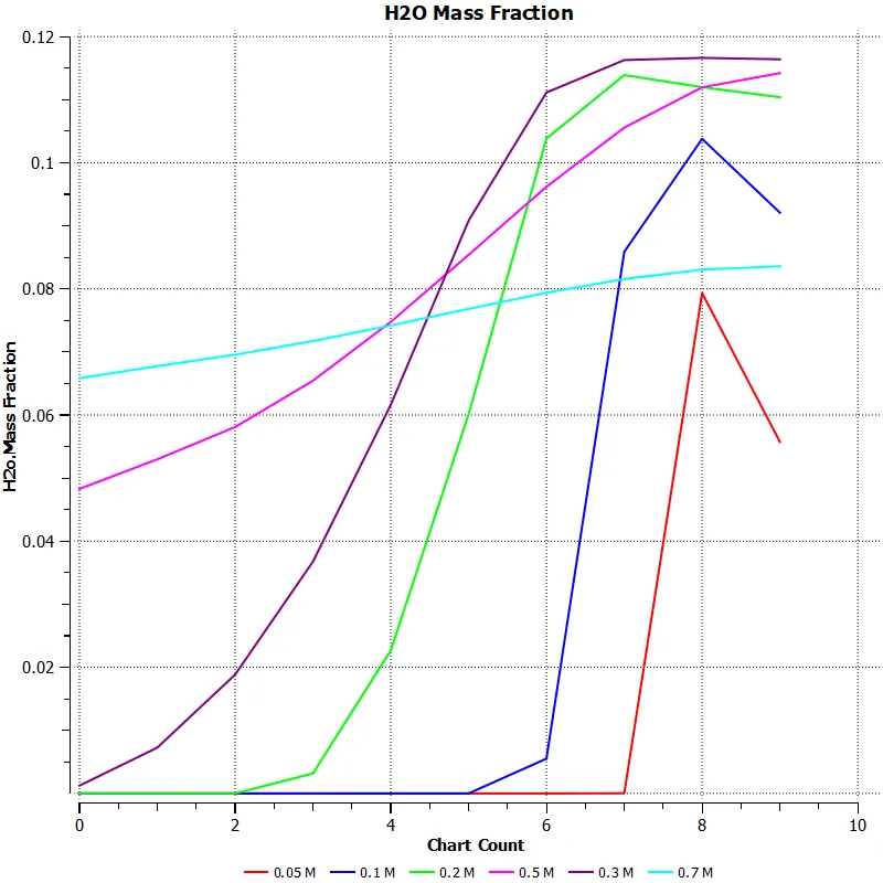
The plot for N2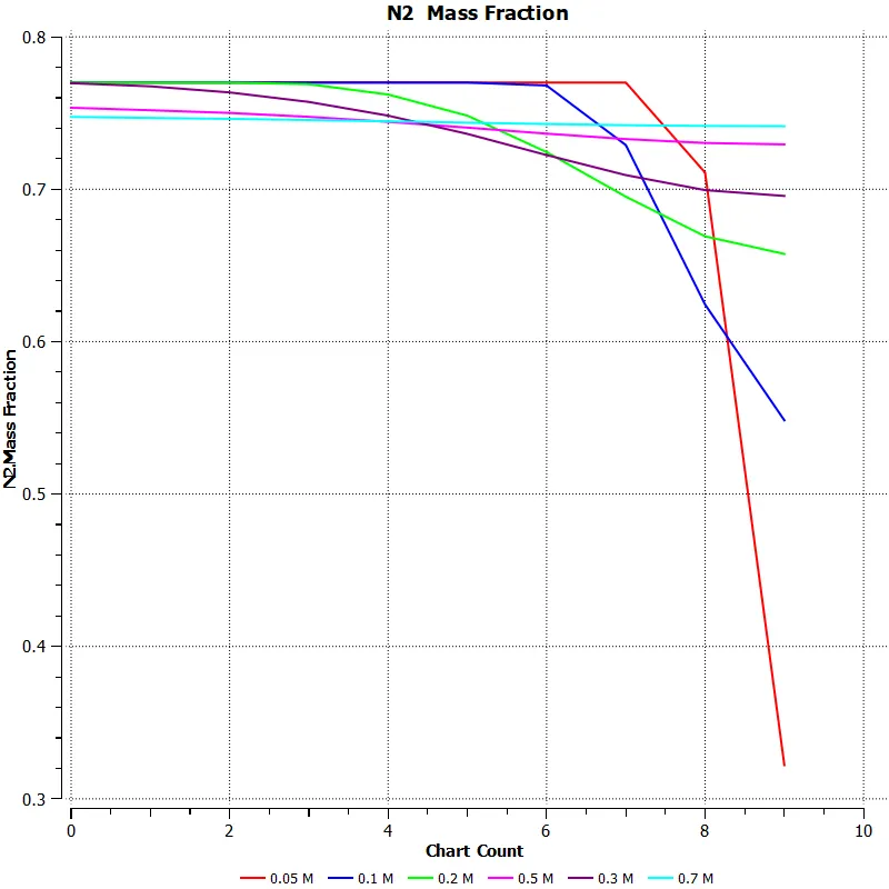
The plots for nox 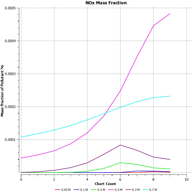
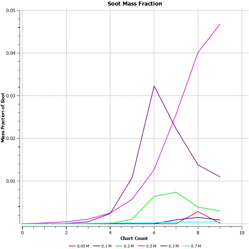
The plots for soot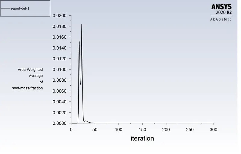
The temperature contour is as shown below 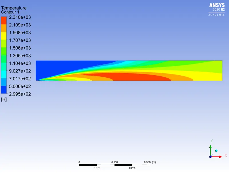
CONCLUSIONS FROM PART 1:
1) From the temperature contour we can see that the highest temperature of 2310K occurs about halfway into the chamber where the air and fuel have had sufficient time to mix.
2) From the CH4 plot, we can see that the highest mass fraction of ch4 occurs near the inlet, as combustion takes place the mass fraction decreases.
3) the highest fraction of Co2 and h20 is at 0.3 m from the inlet, where combustion takes place.
4) From the plot of N2, we can see that the value remains relatively constant, but is least close to the inlet.
5) Oxygen mass fraction is highest near the inlet and is close to zero where the combustion starts.
6)the mass fraction of the pollutants is highest near the end of the model(0.5 m), once combustion takes place.
PART 2: A parametric study of mass fraction of Nox and soot as water is added to the combustion chamber.
To vary the mass fraction of water added into the combustion chamber from 5% to 30 % we run a parametric study, with water and CH4 as the study variables.
An image of the parametric study is shown below.
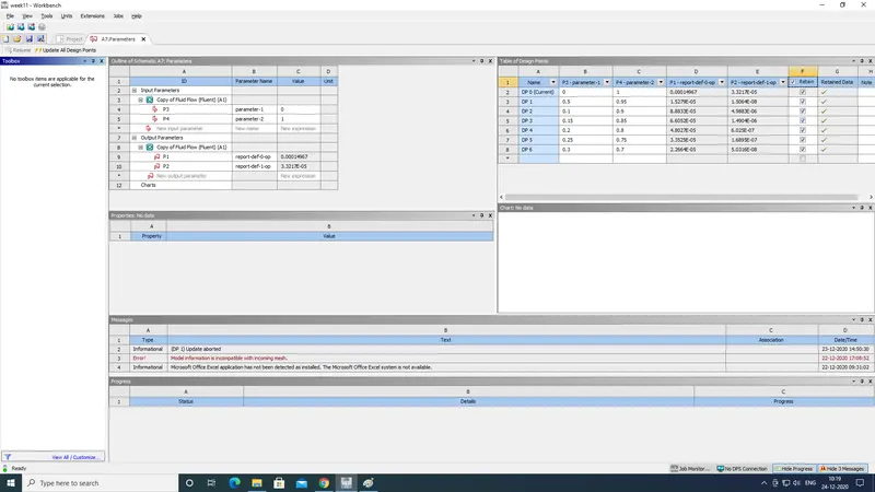
We will analyse each case separately with the related images and plots
case 1: water - 0% CH4 -100%
Temperature contour:
NoX contour: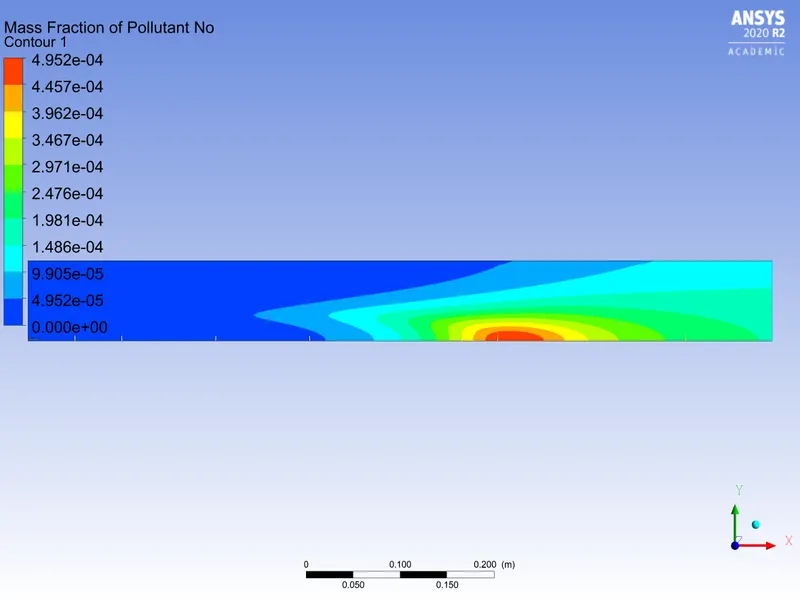
NoX plot:
Soot Contour: 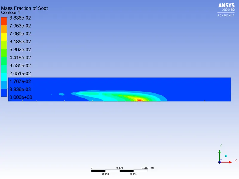
Soot plot :
case 2: water - 5% CH4 -95%
Temperature contour: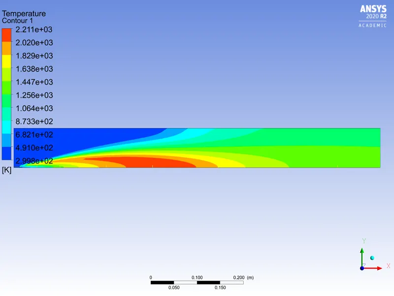
NoX contour: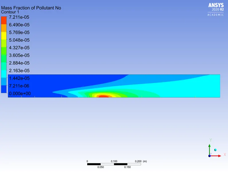
NoX plot: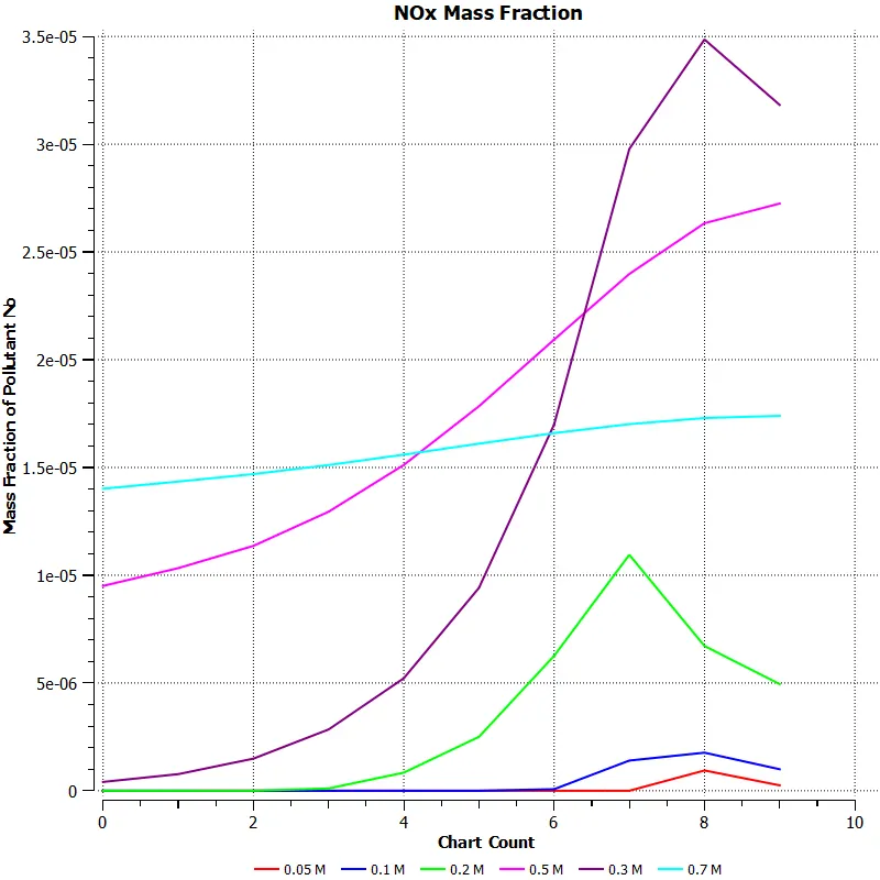
Soot Contour: 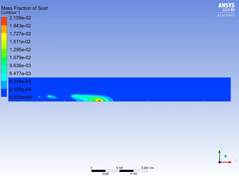
Soot plot :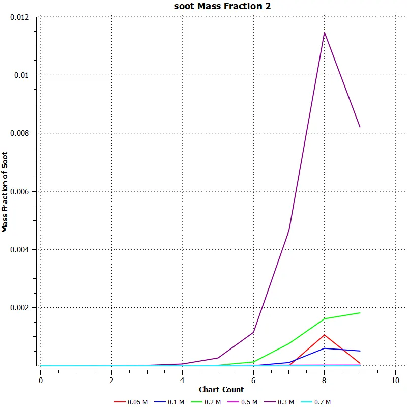
case 3: water - 10% CH4 -90%
Temperature contour: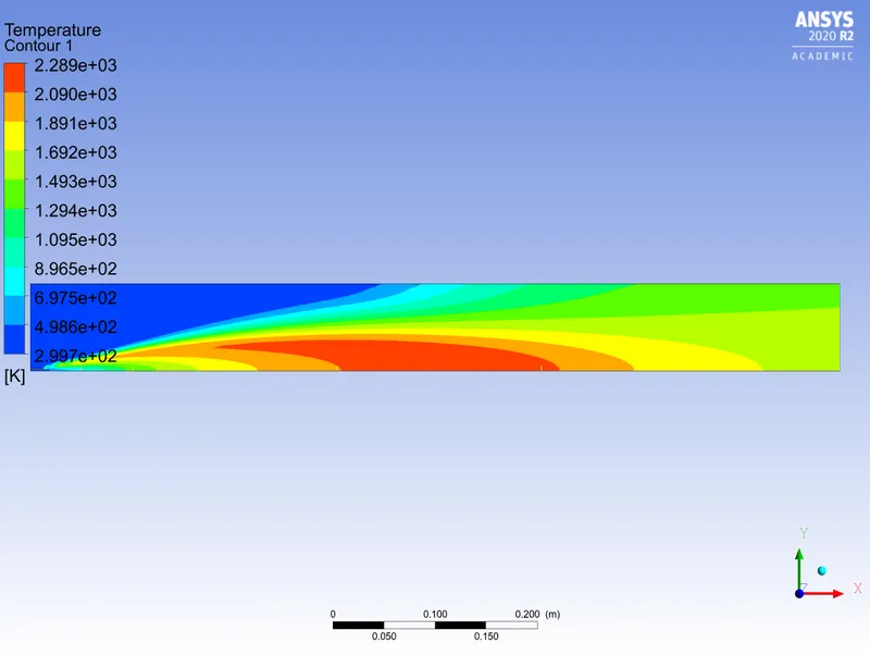
NoX contour: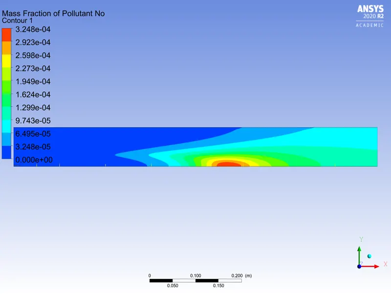
NoX plot: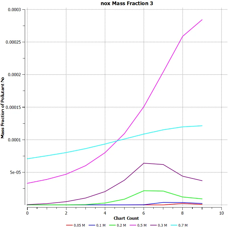
Soot Contour: 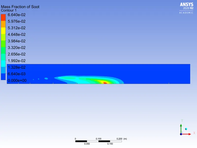
Soot plot :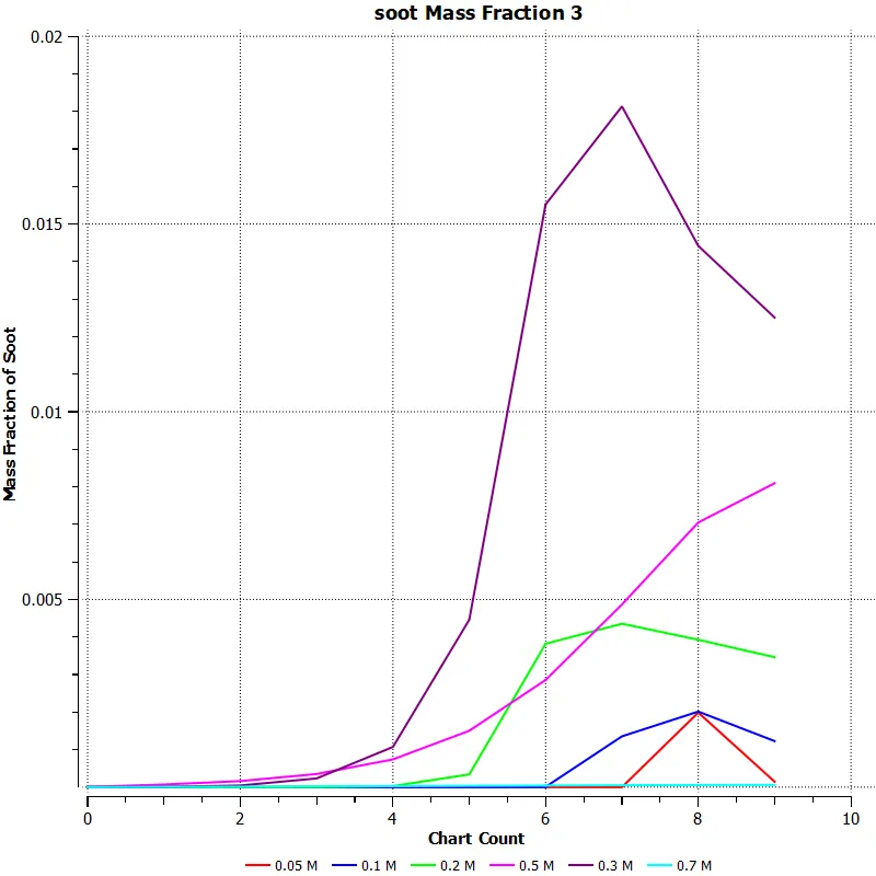
case 4: water - 15% CH4 -85%
Temperature contour: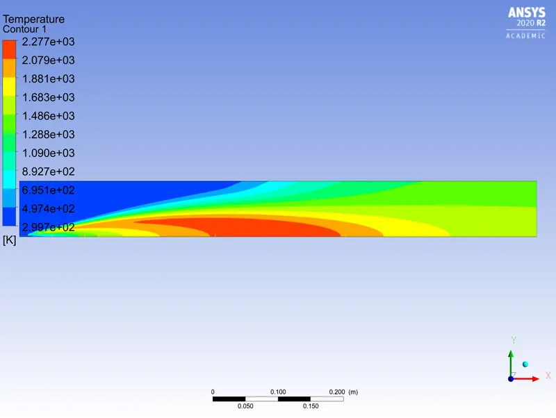
NoX contour: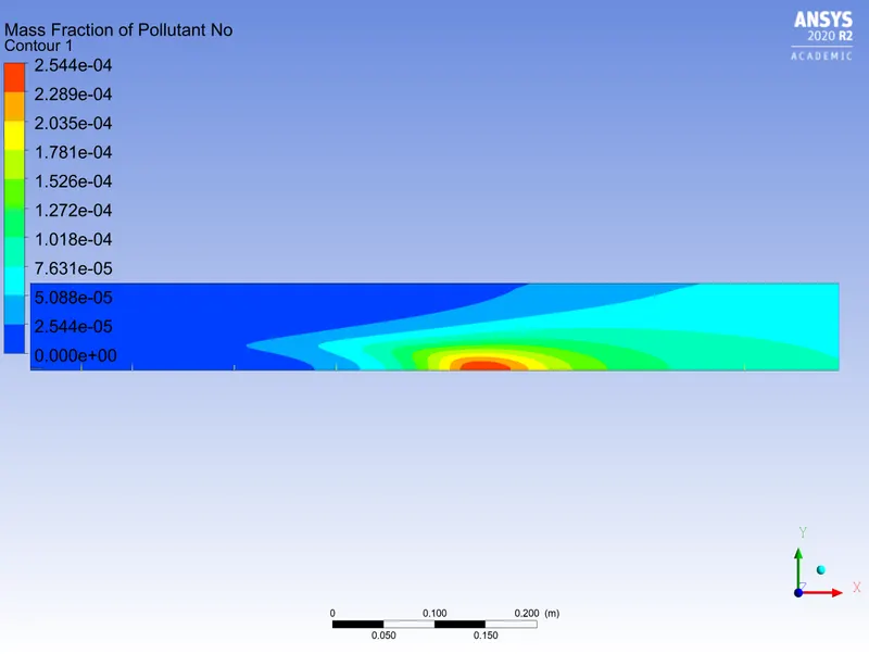
NoX plot: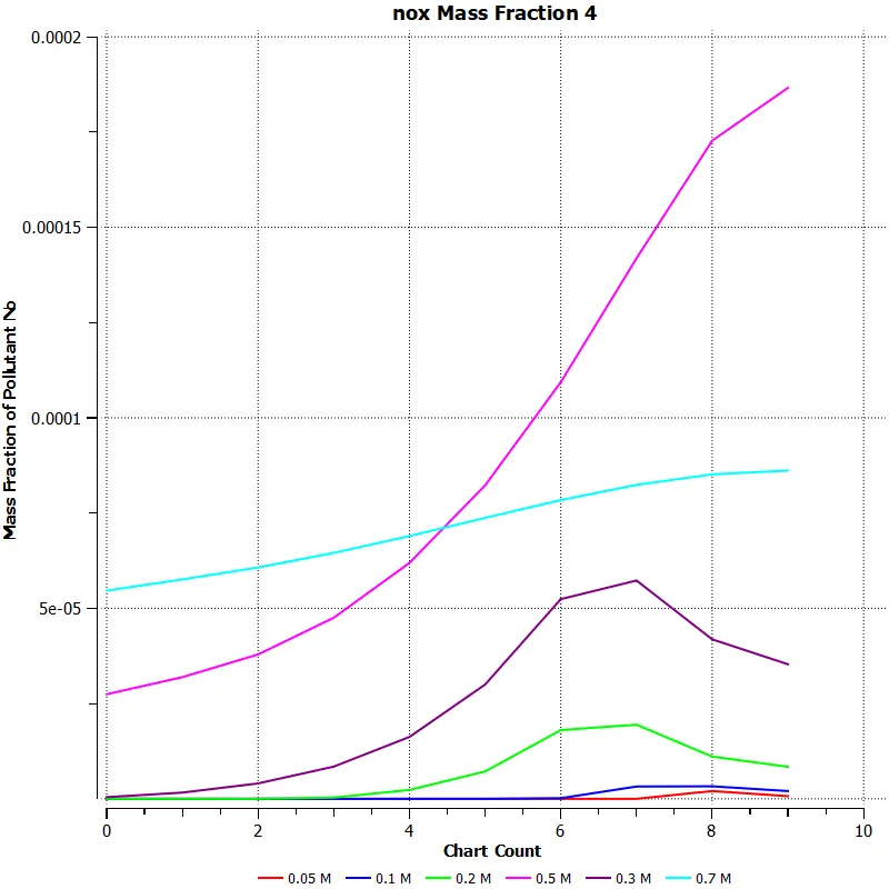
Soot Contour: 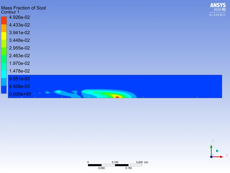
Soot plot :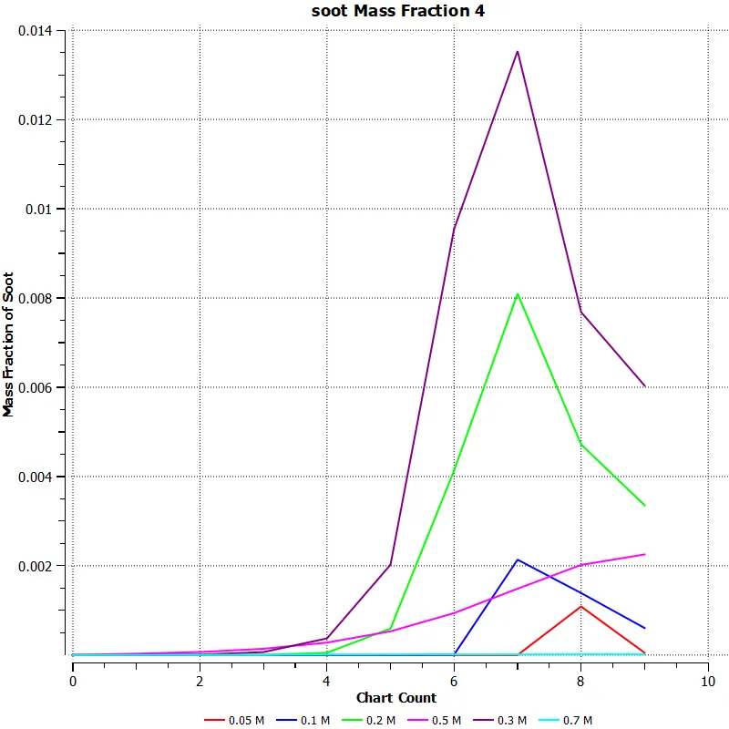
case 5: water - 20% CH4 -80%
Temperature contour: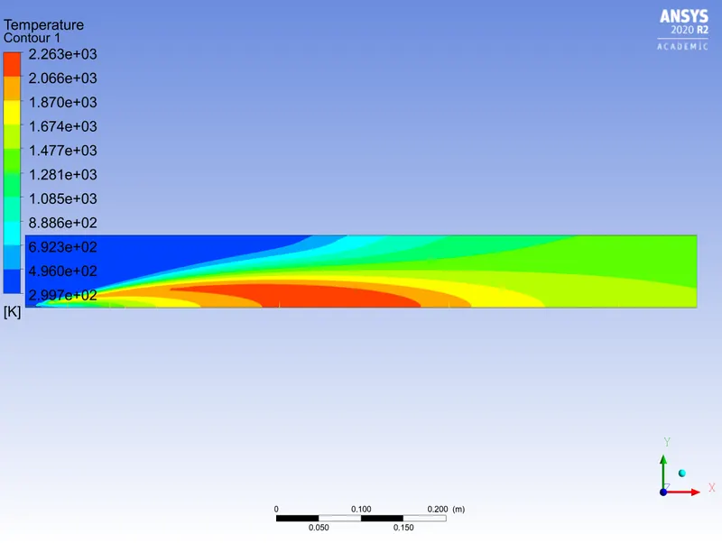
NoX contour: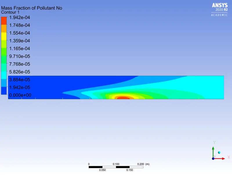
NoX plot: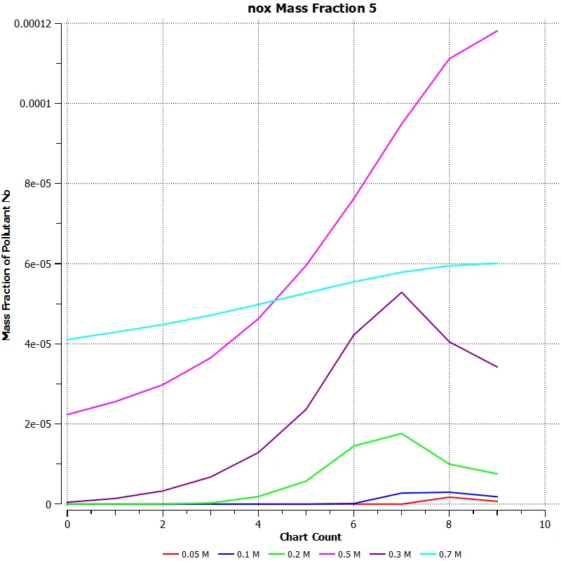
Soot Contour: 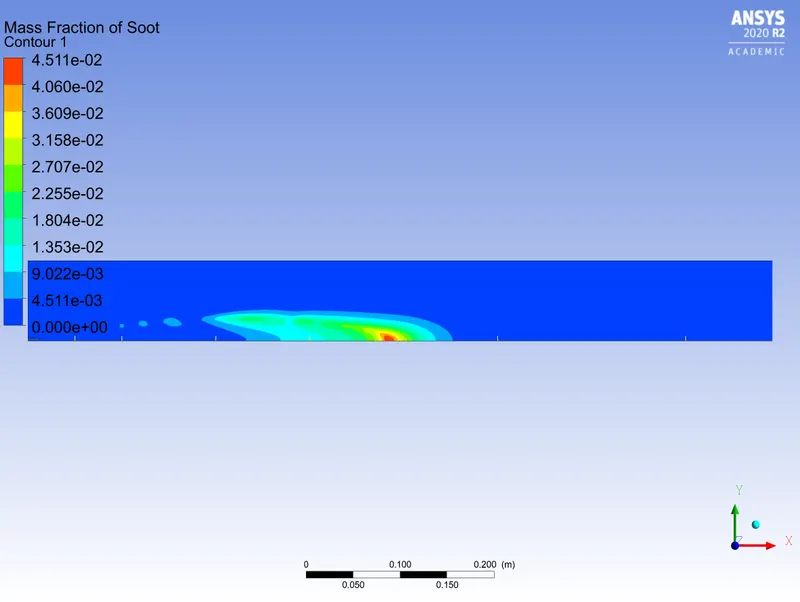
Soot plot :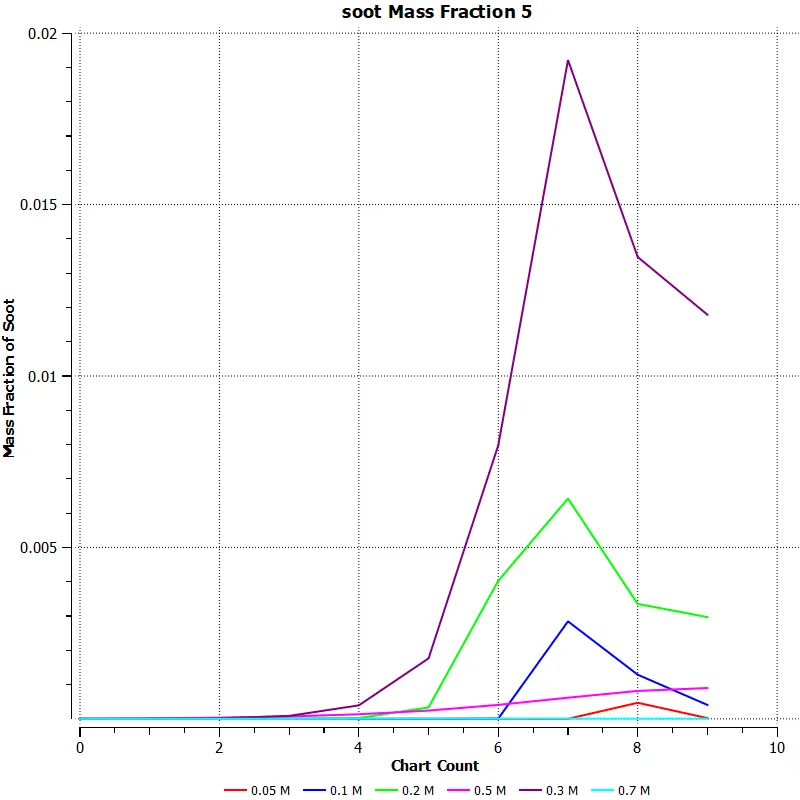
case 6: water - 25% CH4 -75%
Temperature contour: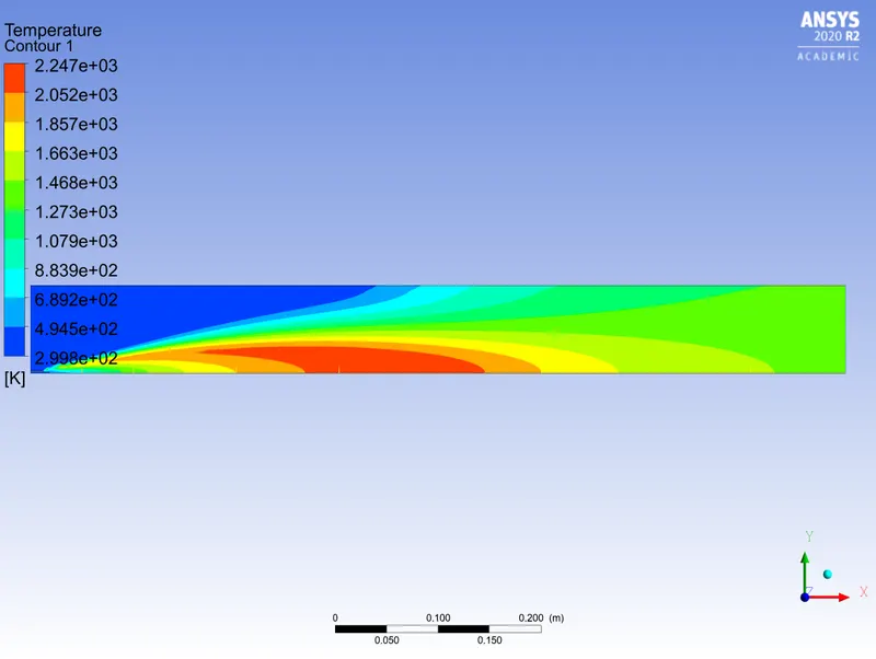
NoX contour: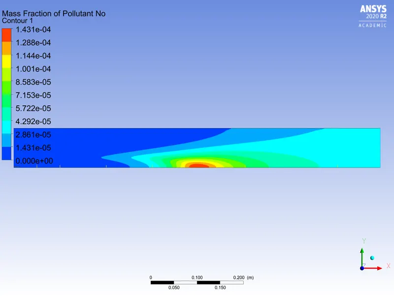
NoX plot: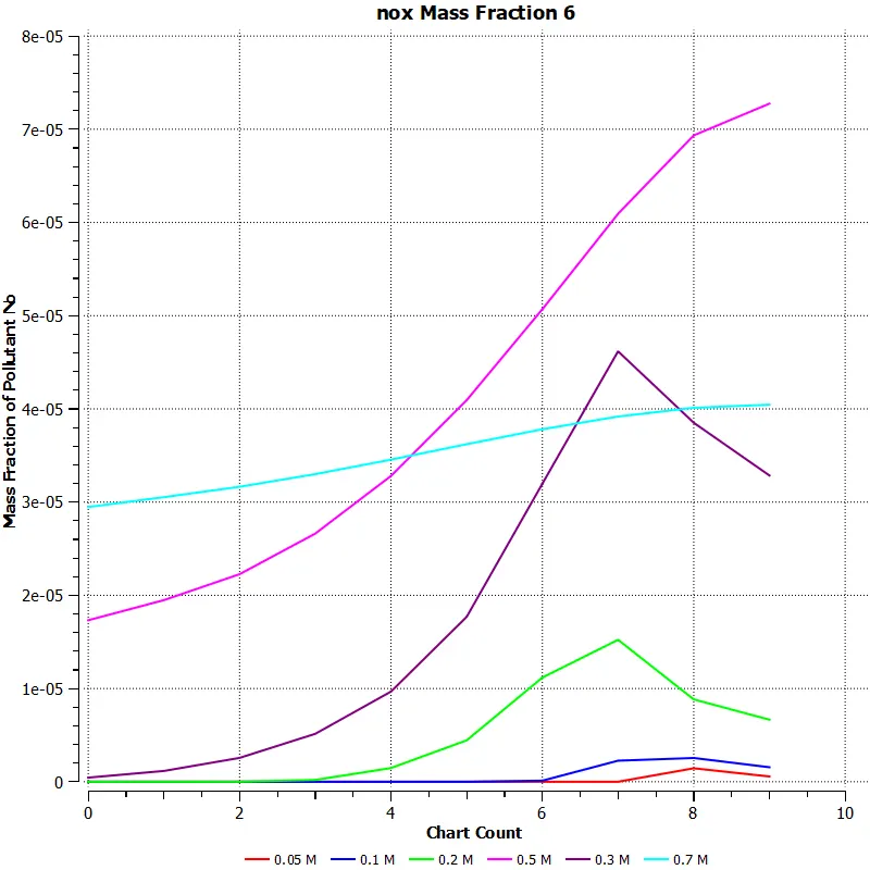
Soot Contour: 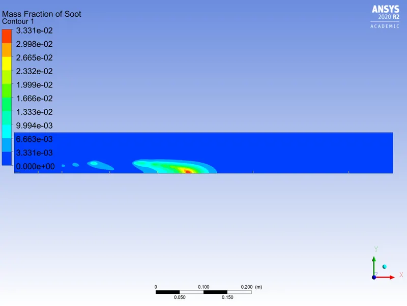
Soot plot :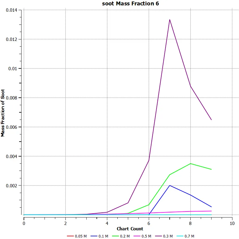
case 7: water - 30% CH4 -70%
Temperature contour: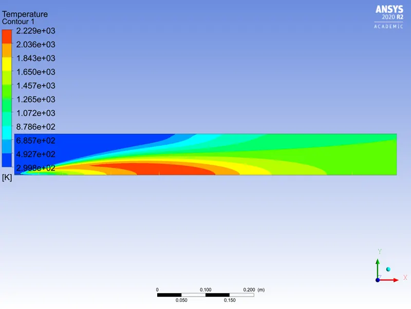
NoX contour: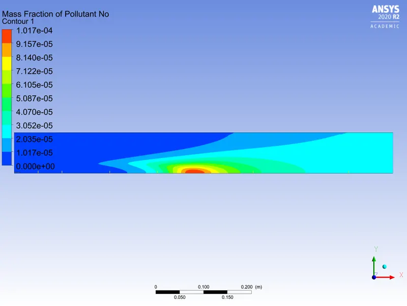
NoX plot: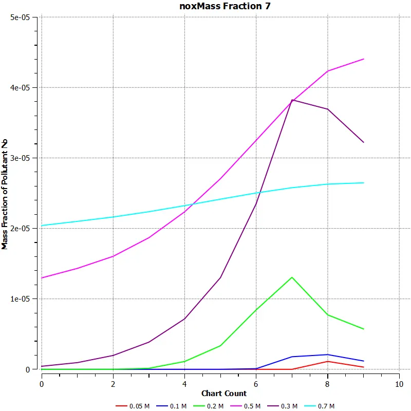
Soot Contour:
Soot plot :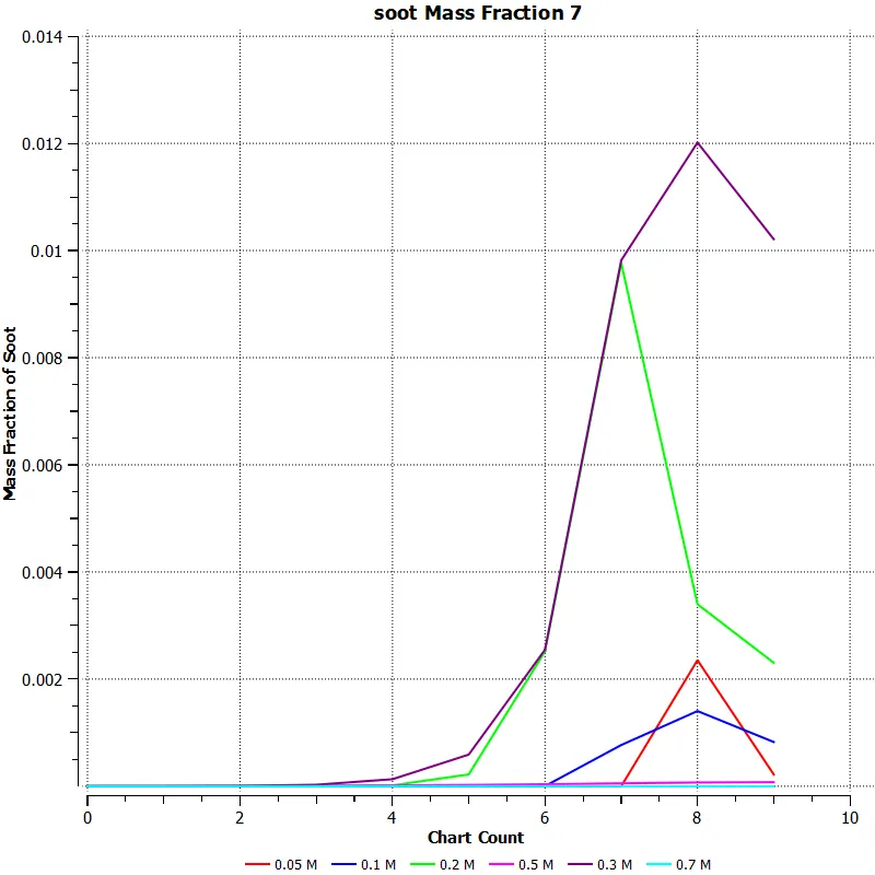
CONCLUSIONS FROM PART 2:
1) The max combustion temperature reduces from 2310k to 2229k
2) No variation in N2 and o2 mass fraction
3) Mass fraction of NoX reduces as water is added to the fuel, from 0.000475 to 4.5e-5
4) Mass fraction of soot reduces as water is added to the fuel, from 0.04 to 0.012
5) From the contours we can see that the max concentration of NoX and soot reduces drastically.