Frontal crash for the Car BIW

Aim:

Car frontal crash analysis using Hypermesh and Hypercrash

Objective:

The objective for the front crash are as follows

1. Check the unit system used in the model and change to either (Mg mm s) or (Kg mm ms)
2. Create the Type 7 interface for the model with the friction value 0.2 and recommended parameters.
3. Check for the interaction and penetrations.
4. Correct rigid bodies if any issues.
5. Create a rigid wall with friction 0.1
6. Compare the model weight with the full-scale 300k nodes model and use added masses to reach the target weight of 700kg while getting CG about the required range.
7. Put the initial velocity of 35mph.
8. Use a model checker to ensure good quality.
9. Time-step :0.5 to 0.1 microseconds.
10. Give Run time for the simulation as 80 ms.

Objectives output requests :

• Create the Sectional force in the rails at the location of the indicated node no. 174247.
• Create the sectional forces that give the Axial force received on the rails from the bumper.
• Shotgun cross-sectional forces.
• A pillar cross-section forces.
• Acceleration curve received on the accelerometer at base of B pillar (on B pillar rocker).
• Intrusions on the dash wall node no.66695,66244.

Methodology :

1. Open the file in Hypermesh and check the unit system used.
2. Create the interface for the crash
3. Create a Rigid wall for the front crash.
4. Add the appropriate amount of mass to the model to obtain the COG at the required location.
5. Create the Initial velocity condition.
6. Check for the errors in the final model.
7. Giving the required time step value and the engine run value.

Introduction:

Crashworthiness is one of the core topics in the passive safety of vehicles and plays an important role in the condition that the impact cannot be avoided. Generally, the analysis of crashworthiness is based on the related crash responses, i.e. the displacement, velocity, and acceleration, of critical parts of a vehicle in full car crash tests. However, these tests are required appropriate facilities, one or more cars with measuring devices, experienced staff, and a long time to prepare. It means they are complicated, expensive, long-lasting, and therefore not easy to realize. This is especially true in the early stage of the vehicle design. Therefore, vehicle designers and researchers made a lot of effort to build numerical models to describe the crash processes

The frontal area of the car is called the crumple zone. Crumple zones work by managing crash energy and increasing the time over which the deceleration of the occupants of the vehicle occurs, while also preventing intrusion into or deformation of the passenger cabin. This better protects car occupants against injury. This is achieved by the controlled weakening of sacrificial outer parts of the car, while strengthening and increasing the rigidity of the inner part of the body of the car, making the passenger cabin into a "safety cell", by using more reinforcing beams and higher strength steels. Impact energy that does reach the "safety cell" is spread over as wide an area as possible to reduce its deformation.

Reducing the effects of traffic accidents on the occupants is a major objective of collision attempts. Impacts between the car and the pole are very dangerous for the physical integrity of the car’s occupants. To minimalize the effects of such events on the passengers of a vehicle, a whole series of efforts by both designers and experienced engineers led to increasing the vehicle’s safety.

Procedure :

Step 1: Opening the file and checking the Unit system.

The Starter file (.0000 rad ) is imported into the Hypermesh window. To import the file

File >Import>solver deck>import the 0000.rad file.

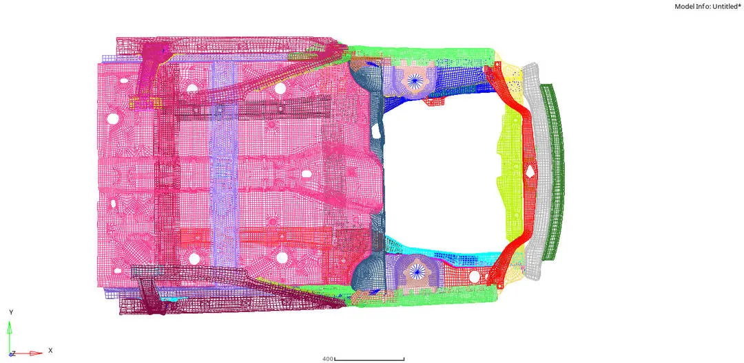
Fig- front crash car BIW

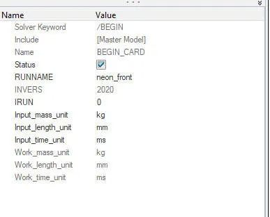
Now it’s important to ensure that the model follows a certain unit system. To check the unit system for the current model.

Model browser> cards >begin_card

Step 2: Creating the interfaces

Type 7 is a general-purpose contact used for most of the contact conditions.

This works on the Penalty method which states that when the slave mode enters or touches the gap of the Master node, a spring element or resistive force is created a the point of contact.

And the reaction forces are then calculated by the solver when the contact develops based on the initial velocity and initial parameters. Also, the time step is decided based on the spring element.

In type 7 the energy jump induced by a node impacting from the shell edges is removed by the use of a cylindrical gap around the edges.

The advantage of Type 7 is that stiffness is not constant and increases with the penetration preventing the node from going through the shell mid surface.

To create the Type 7 interface

Open the Groups in the model browser > right-click on it > Create > rename it to Type 7.

Now choose the Slave entities as the components and select the components. Then choose the Master entities as the components and select the components.

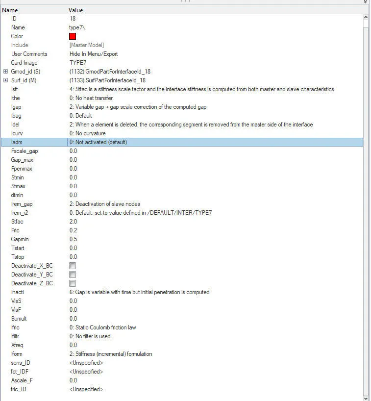
Some important criteria used under the type 7 interface.

Istf- 4 (interface stiffness calculated from both master and slave node characteristics )

Igap- 2 - variable gaps (how the gap size is calculated)

Idel- 2 (element deletion )

Gap_min - 0.5 (to decide the minimum gap to activate the interface condition )

Irem_gap- 2 (deactivation of slave node if element size is lesser than the gap values )

Inacti - 6 (action to take if intial penettration exist)

This Inacti is one of the crucial criteria that helps to decide the steps to take in case the penetration has occurred with the master node.

Now why this penetration has to take care of? The answer is to avoid the unstable run due to the time step.

The time step is calculated as

Delta T=0.5(g-p)/(dp/dt)

g- gap thickness

p- penetration

dp/dt= speed of sound through material.

Now if the g<p, the numerator value will be negative that in turn cause the time step value to be negative. This negative time step will cause an unstable simulation run.

So, the Inacti criteria push the node to the point using some form scale factor multiped with the gap thickness of the master node.

Iform - 2 (friction formulation)

Step 3: Creating the Rigid wall

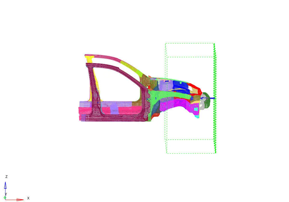
The Rigid wall as the name suggests that it is rigid and not deformation occurs. It is created in order to provide the wall for the slave node beyond which they are not allowed to go.

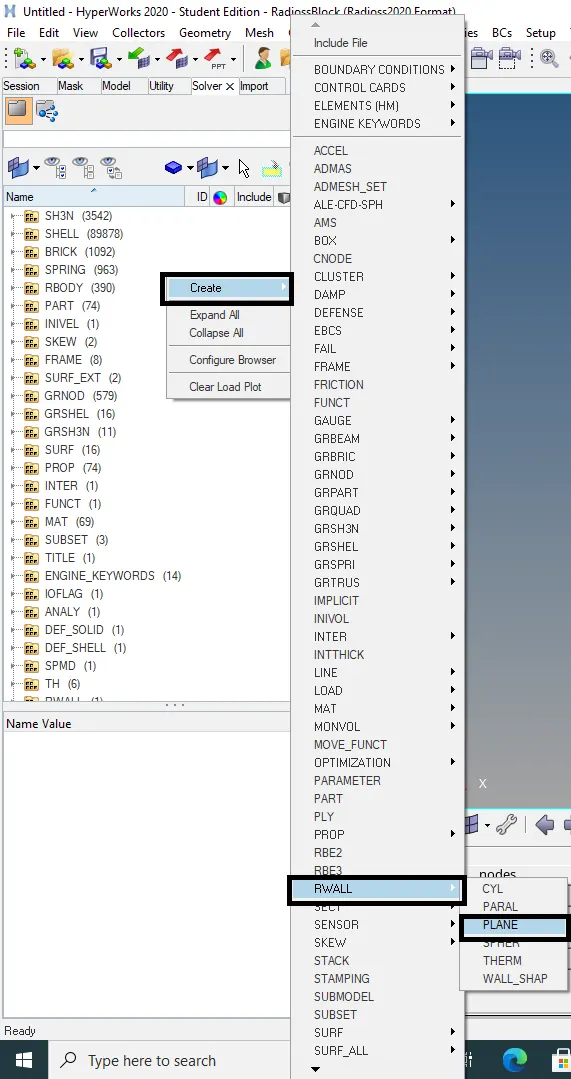
To create the Rigid wall open the Solver browser.

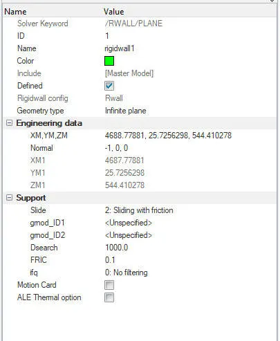
In the solver browser Right click>> Create >> Rwall >>Plane. A new rigid wall card is created, under which insert the required values.

Select the geometry Type as the Infinite plane

Click on the XM, YM, ZM(X, Y, Z coordinates as base node M)> Select the node at the plane rigid walls need to be created.

Select the normal at the axis and based on the direction of normal give a minus(‘’-”) sign in the X direction (see the global coordinate )

Give the Slide value as 2

Friction value as 0.1

Dsearch distance as 1000

Step 4: Reach the model weight to 700kg and Obtain the COG.

The COG of the model is calculated based on the total mass and its distribution over the model.

Here the overall weight of the model has to be matched around 700kg. In order to add the mass in the model.

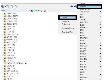
In Solver Browser >>ADMAS>>Right click>> Create. A new add mass card is created and rename it to the appropriate name.

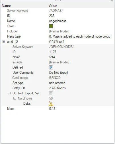
Under the card Select the mass type as 0( mass is added to each node separately ).

Select the gnd_Id >> select the entities id>> nodes. Select the nodes and add the mass value to be added on the nodes selected.

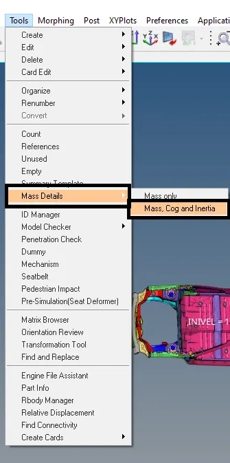
Now check the Total mass and the COG of the model. To check the mass and cog go to Tools>> Mass details >>mass, cog, and inertia.

Maintain the Cog at the appropriate location and match the total mass to 700 kg.

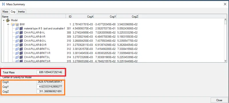
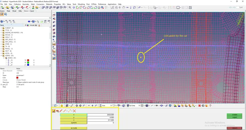
Plot the obtain Cog point in the model.

geometry>nodes > create

Step 5: Create the initial velocity.

Initial velocity has to be applied to the car model with which it will impact the rigid wall. To create the initial velocity.

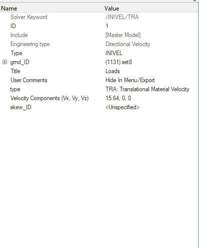
Solver browser > right-click>>create >> Boundary conditions>> select the INVEL>> give the card a name.

Under the card,>create the gnd_id>> select the entities _id as nodes by displayed and proceed.

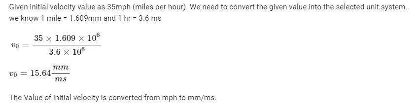
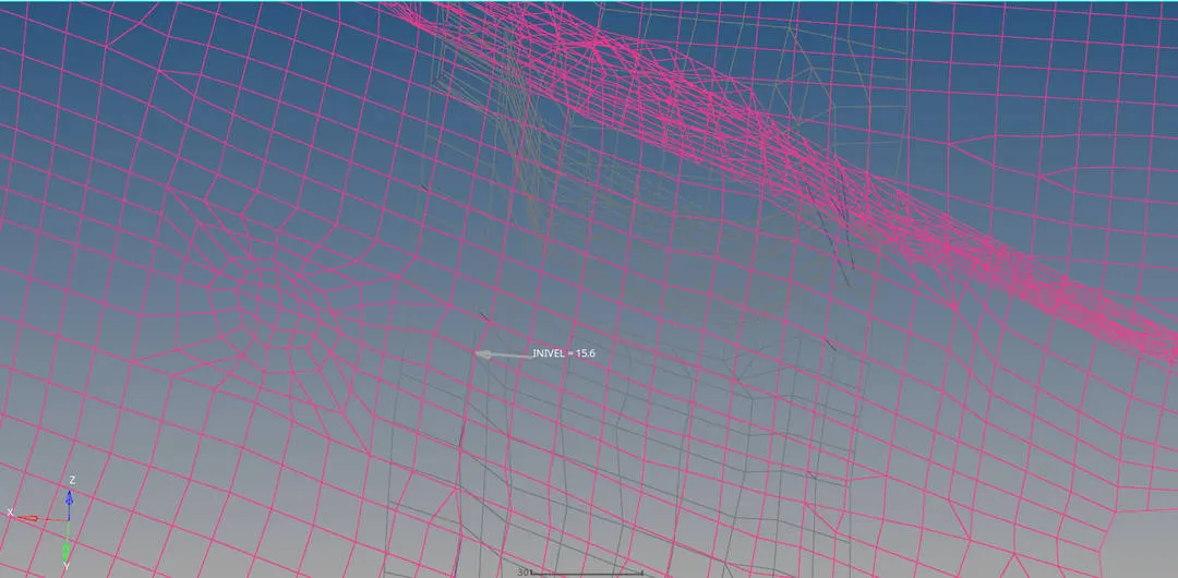
Enter the Velocity value in the direction to be applied. Here the velocity is apple at the X direction 15.64.

Step 6: Creating the sections :

The section is created at a particular part in order to see the distortion and stresses in this section.

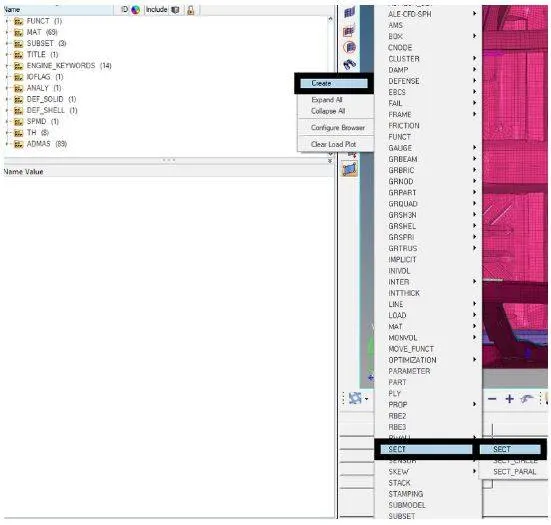
To create the section go to the Solver browser >>right-click>> create >> SECT>> In the entity Editor, give the N1, N2, N3 as the nodes >> a skew is created at this location.

After that, we need a local coordinate system for this section. For that, we create the Fram.

Create >>Frame >> select the node in the same direction as selected for the section.

Now go to the section card earlier created >>Frame_id >> select the frame system as created above.

Enter the Delta T value as 0.1 and alpha value as 1.67.

Under the Grshell_id >> right-click >> create >> select the entities _id as elements on the area where the section is created.

Iframe as 12 i.e On cog

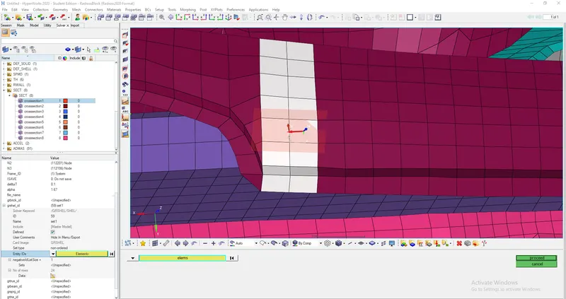
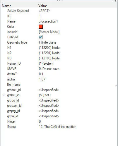
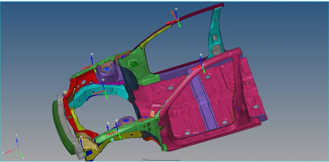
Fig- Section for all the parts

Like these, the section is created at the Shotgun, bumper rails, and headlight fender.

Calling the section in the output :

The section created needs to be called at the output so that it can be analyzed.

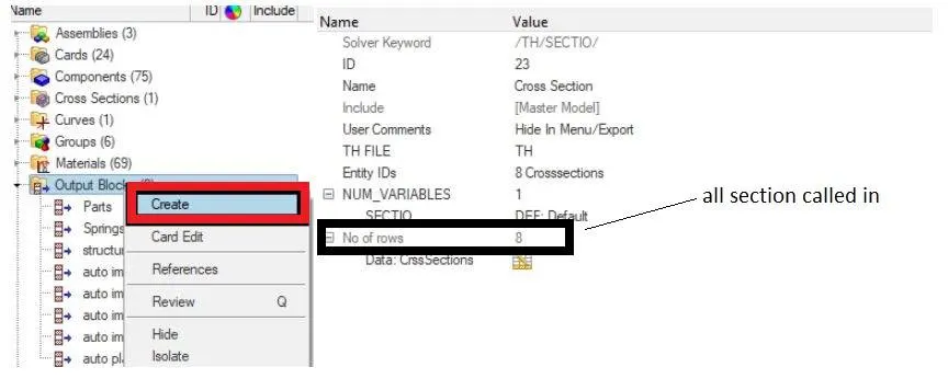
To call out the Section. Model browser >> Output blocks >>right-click>> create >> rename it to the cross section.

Select the Entity_id as Cross-section and the cross-section is done.

Step 7: Creating the accelerometer:

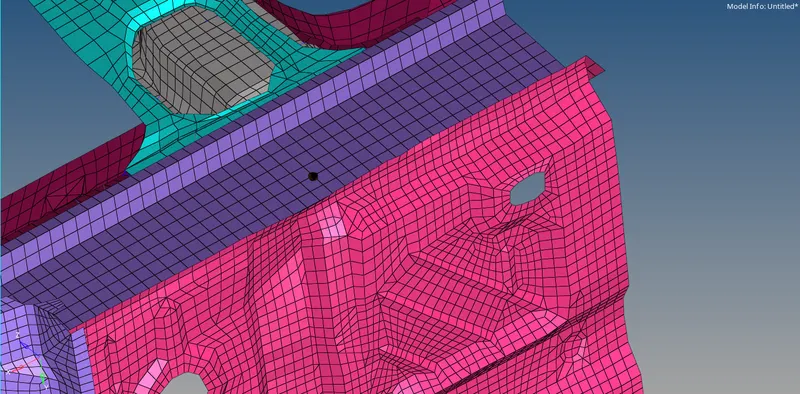
The accelerometer is created at the two Rockers of the Car BIW.

To create an Accelerometer on the rocker box below the B pillar.

Goto > Tab bar > solver browser > right click and create > Accelerometer.

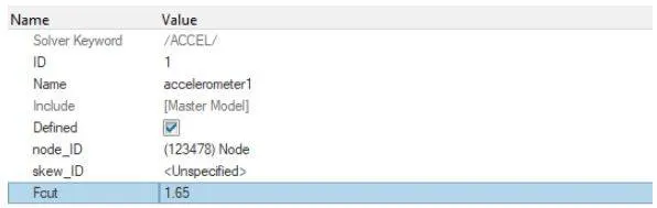
Select the node_id and enter Fcut=1.65.

So another accelerometer is created at the side rocker also.

Calling the section in the output :

The accelerometer created needs to be called at the output so that it can be analyzed.

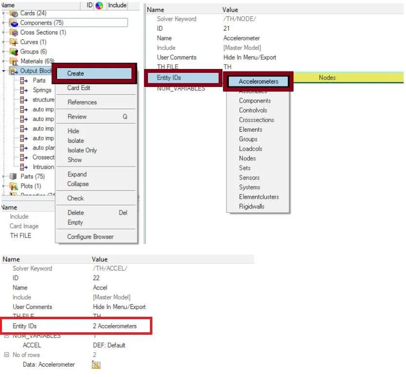
To call out the accelerometer. Model browser >> Output blocks >>right-click>> create >> rename it to the accelerometer.

Select the Entity_id as an accelerometer which was created at the two rockers.

Step 7: Creating the intrusions :

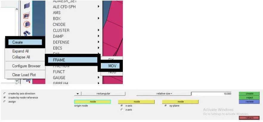
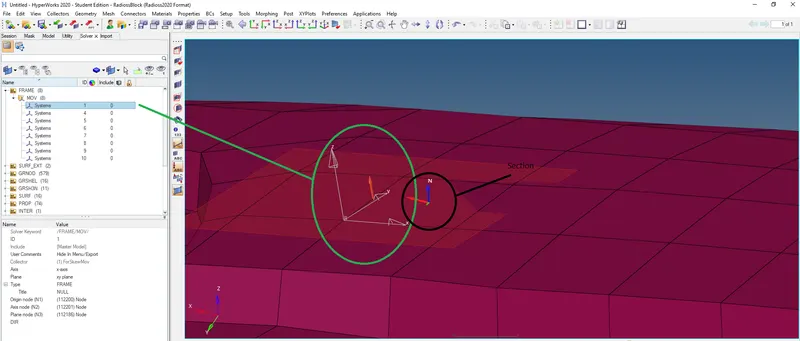
To create the intrusions at the specific node location, first, we need to have a Moving Skew.

Go to the Solver Browser >> right-click>> Create >> skew >> mov

Select the nodes as origin, axis, planes.

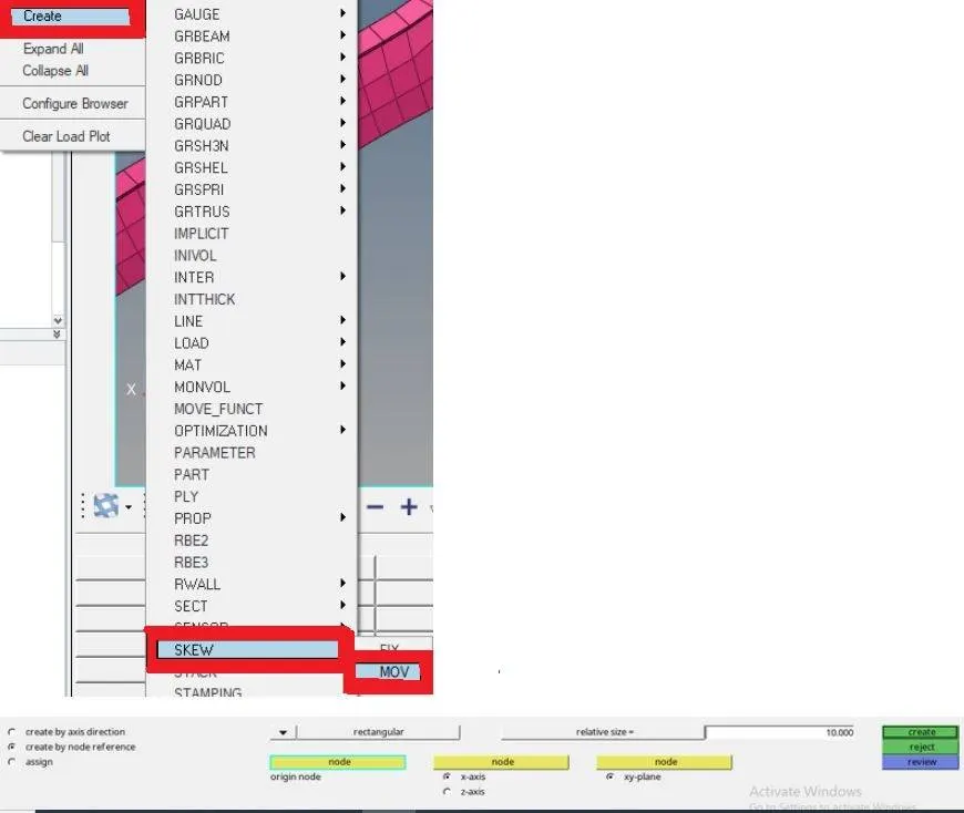
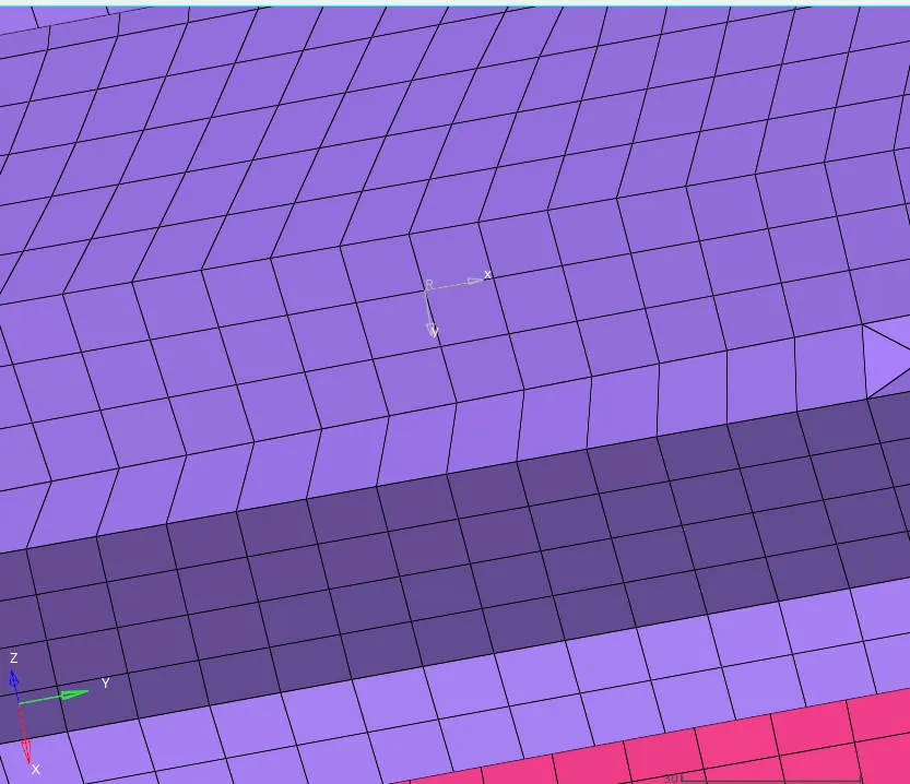
The skew should be created in line with the node taken for the intrusion.

This intrusion is created in the output_blocks.

Model browser >> Output_blocks >> right -click>> create >> name it to intrusion 1

Select the Entity_id as a node

Node >> by id >> type 66244>> proceed

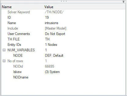
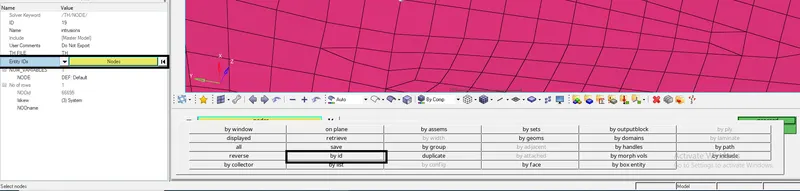
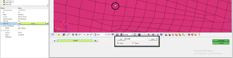
Then select the Iskew as the skew mov created earlier.

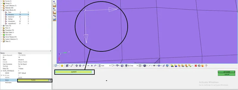
Same way for the other node the intrusion can be created.

Step 8: Check for the penetrations :

The model has to be checked for the penetrations if there are two components elements are penetrating with each other.

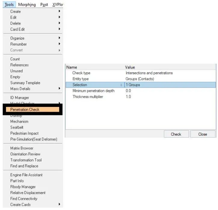
To check for the penetrations, go to the Tools menu >> Penetrations check >> in the entity editor, click on the selection and click on the group>>Give the group. >> check

There is no penetration found in this model.

Step 9: Checking for the errors :

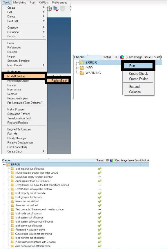
The model has to checked for errors if there are any errors and incompatible conditions present.

Menu bar >>Tools >> model checker >>radioss block

Step 10: Giving the time step and run time values :

After the Model check is done, apply the time-step value tfreq=0.5.

Goto > Tab bar > cards > ENG_ANIM_DT.

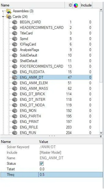
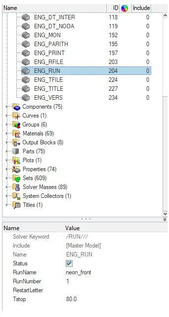
After editing the time step, apply the run-time value Tstop=80.

Goto > Tab bar > cards > ENG_RUN.

Basic steps for simulation :

• Import the starter file (rad_0000) into the Radioss block
• Provide the proper material and failure to the component(Rupture plate). Since here it’s already provided with Law 2 as material and failure Johnson card.
• Then go to Analysis > Radioss> load the starter file > radioss. Simulate with no errors.

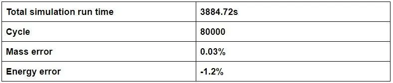
• Open the output file (rad_0001) to check for the energy error(less than 15%) and mass error(less than 1%).
• Now open the Hyperview and check the simulation using H3d file
• Open the Hypergraph 2D to observe the energy plots with the T01 file.

Errors faced :

The errors are shown while the simulation is run though these errors are not shown in the Hypermesh Radioss block Model checker. For this, the File is exported and then opened in the Hypercrash to

check for the errors and eliminate the errors.

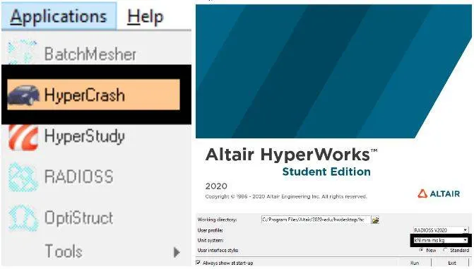
To open the Hypercrash go to Applications in the Menu bar >> Hypercrash. Then the Hypercrash windows open >>file >> import the RAdioss file.

Go the Quality >>model checker >> run

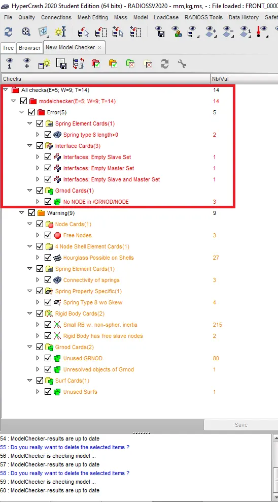
These errors include the spring card, interface empty, and Gnod empty cards. The spring card can be deleted because as such there is no spring used in this model. For the interface and Gnod, this all can also be deleted.

Empty cards are created while selecting the nodes empty cards are created which creates issues in the final simulation process.

Then the file is again exported and again Opened in the Hypermesh. Before running the simulation the open the cards and delete the Unsupported cards. The unsupported cards are created while the file exported to the Hypercrash and this

card also shows as the error in the simulation, so it's necessary to delete the card.

Results :

Simulation :

The animation shows the deformation is taking place at the frontal area and it is then passed to the rear end of the car. The impact is taking place in the frontal area and the focus is to save the driver seat but the impact more and the passenger cannot be saved in this impact.

The plastic strain means that the element has deformed and absorbed the forces. It shows the good sign that the plastic strain is only formed in the frontal area of the car and not to the rear end of the car.

Graph plotting:

Energy plots :

Observations for energies:

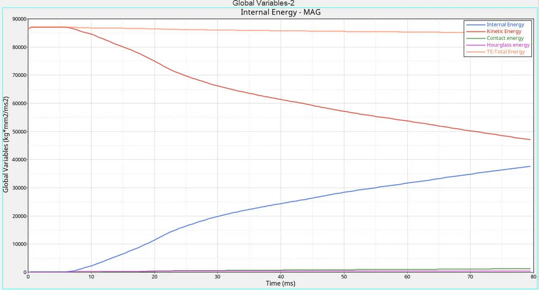
The energy plot for internal, kinetic, total along with the hourglass and contact energy is shown in the above graph. The hourglass energy is very minimal in this case which is a good sign. This is due to the use of good shell formulation here QEPH shell which has a good amount of integration points that helps in reducing the hourglass effect.

Taking about the contact forces here it is also very minimal and somewhat linear which means a good sign. Also, the contact forces and hourglass energy has to be less than 15% of the total energy which the graph shows as a needed result.

The kinetic and internal plots show the mirror image. That means the decrease in kinetic and an increase in internal energy at the same time. This graph shows the total energy as an almost straight line because it is the summation of the kinetic and internal energy.

A-pillar crosssection forces :

right left

Bumper crosssection forces:

right left

Shotgun crosssection forces:

right left

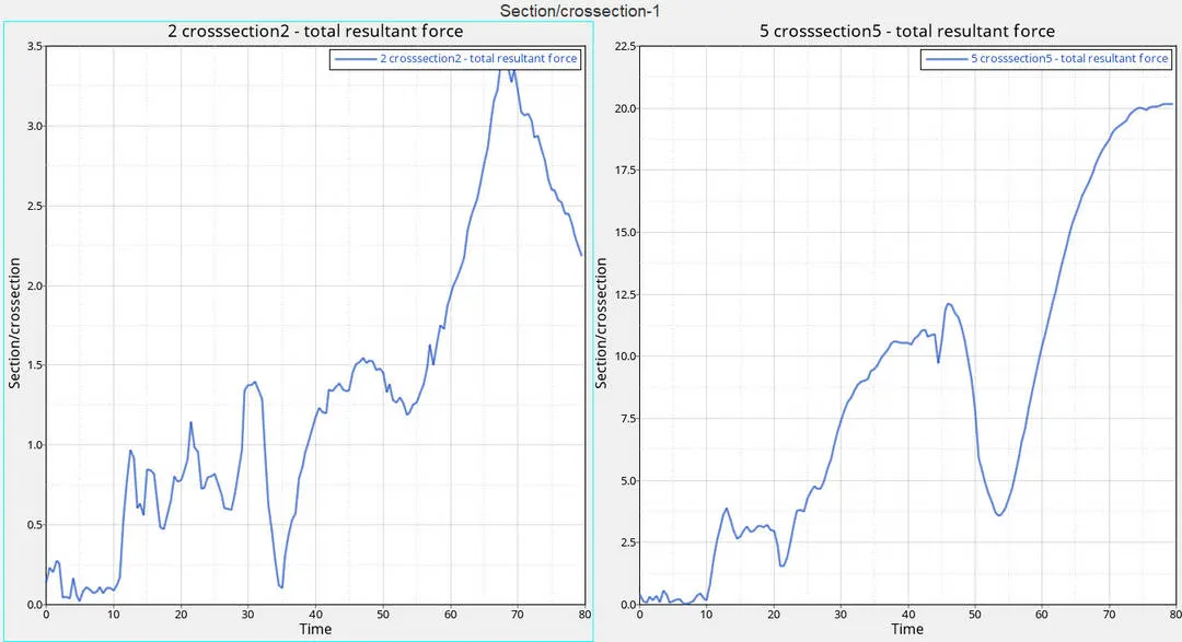
Rails crosssection forces:

left right

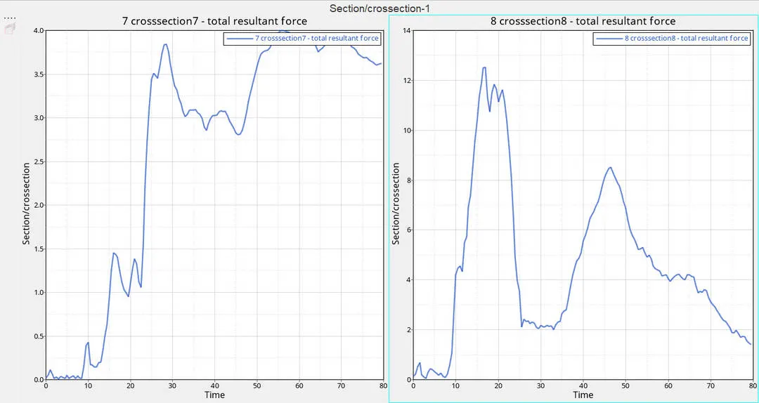
Observation for crosssection forces:

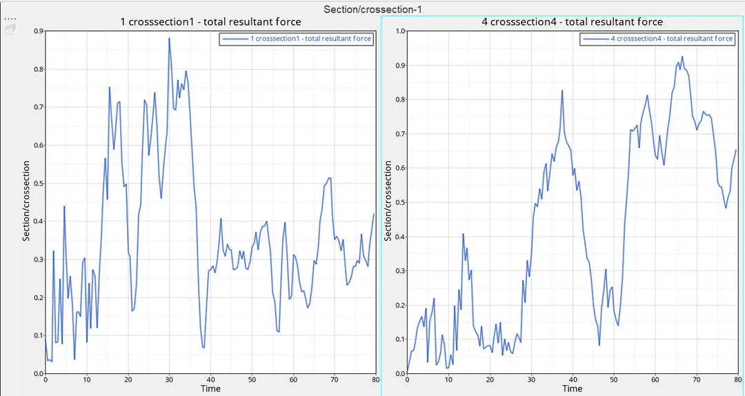
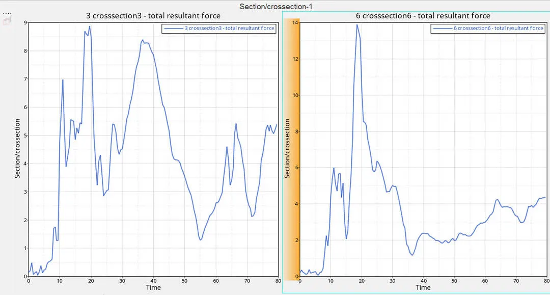
If we see closely the section forces for all the parts, the parts to the right side have higher forces value at the particular as compared to the parts on the left side.

The force values in the graph fluctuate, it goes higher then drops to the lower values than peaks to higher values.

From the graph, the shotgun part shows the maximum amount of the resultant force followed by the bumper then rails, and lastly the A-pillar.

A-pillar shows a very minimal amount of forces as compared to the other components around 0.9 to 1.0

Intrusions :

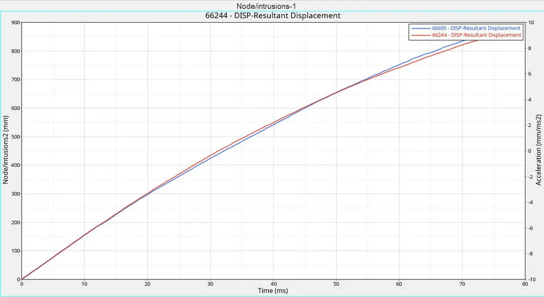
The intrusion curve shows the linear increase of displacement of the node with respect to time for the moving skew for both nodes.

It is noted that the distance between the initial skew and final skew changes from 800mm to 900mm after the crash at time 80ms.

Accelerometer:

Left Right

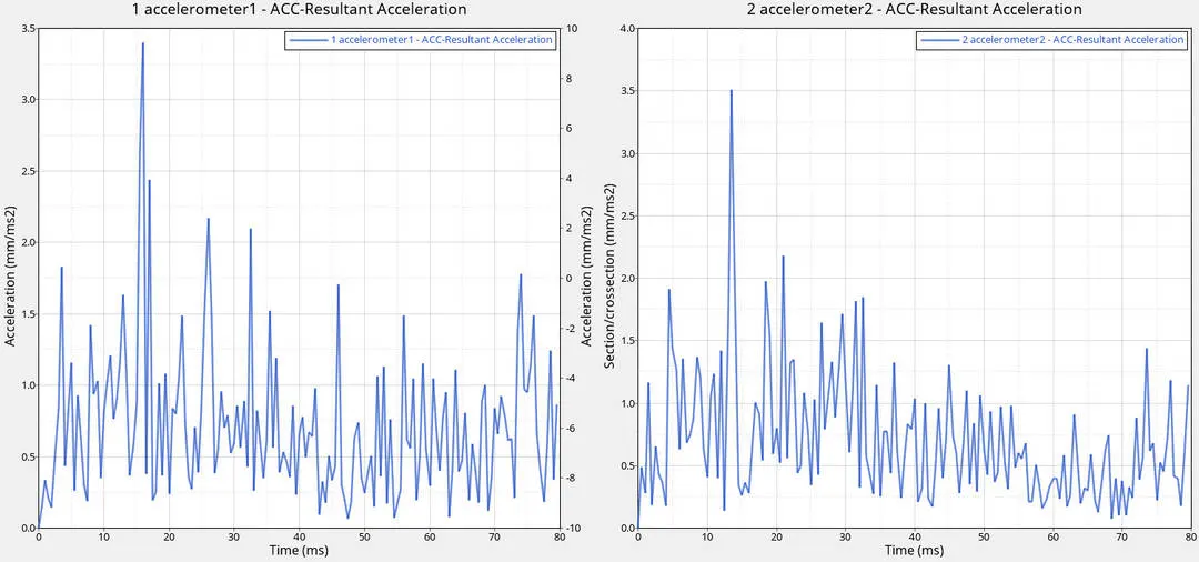
An accelerometer is used to measure the acceleration in the component (change in velocity with the time ). The graph shows very much fluctuations in the acceleration values with time. This fluctuation is due to the noise present in the body i.e some unwanted vibrations.

The max value for the left side component peaks at around 3.4mm/ms^2 and for the left side, it is 3.5mm/ms^2.

In acceleration, the term Fcut =1.65 is used which means vibrations frequency is cut to obtain the smooth plot. But value might not be that significant in avoiding the vibrations.

Conclusion :

The frontal crash for the car was carried with all required outputs such energies plot and the intrusions successfully.