Week 4.1 - Genetic Algorithm

Aim:

Understanding the genetic algorithm for optimization the stalagmite function

Objective :

• Write the code to optimize the stalagmite function.
• Explain all the ga syntax.
• Plot the graphs for all the 3 cases.

Introduction :

Genetic algorithm:

A genetic algorithm is a search heuristic that is inspired by Charles Darwin’s theory of natural evolution. This algorithm reflects the process of natural selection where the fittest individuals are selected for reproduction in order to produce offspring of the next generation.

Notion of Natural Selection
The process of natural selection starts with the selection of fittest individuals from a population. They produce offspring which inherit the characteristics of the parents and will be added to the next generation. If parents have better fitness, their offspring will be better than parents and have a better chance at surviving. This process keeps on iterating and at the end, a generation with the fittest individuals will be found.
This notion can be applied for a search problem. We consider a set of solutions for a problem and select the set of best ones out of them.
Five phases are considered in a genetic algorithm.
Initial population
Fitness function
Selection
Crossover
Mutation

Governing equations :

General syntax for the ga:

x = ga(fun,nvars)
x = ga(fun,nvars,A,b)
x = ga(fun,nvars,A,b,Aeq,beq)
x = ga(fun,nvars,A,b,Aeq,beq,lb,ub)
x = ga(fun,nvars,A,b,Aeq,beq,lb,ub,nonlcon)
x = ga(fun,nvars,A,b,Aeq,beq,lb,ub,nonlcon,options)
x = ga(fun,nvars,A,b,[],[],lb,ub,nonlcon,IntCon)
x = ga(fun,nvars,A,b,[],[],lb,ub,nonlcon,IntCon,options)
x = ga(problem)
[x,fval] = ga(___)
[x,fval,exitflag,output] = ga(___)
[x,fval,exitflag,output,population,scores] = ga(___)

The Function is for the Genetic Algorithm of the global minima but in order to attain the maxima value the ‘-’ is placed before
the equation.
Where,
The Global maxima is as follows
f(x, y) = f1 . x × f2 . x × f1 . y × f2 . y

where ,
`f1 . x = [sin(5.1πx + 0.5)]^6`
`f1 . y = [sin(5.1πy + 0.5)]^6`
`f2 . x = exp[ − 4 ln(2) ×(x − 0.0667)^ 2/0.64]`

`f2 . y = exp[ − 4 ln(2) ×(y − 0.0667)^ 2/0.64]`

Process of Solving:
The Order in which the code is written is as below
1. Write Stalagmite Function.`f(x, y) = f1 . x × f2 . x × f1 . y × f2 . y f1 .
2. Evaluating the stalagmite function.
3. Writing the code for Unbounded Inputs.
4. Writing the code for the Bounded Inputs.
5. Writing the code for the Bounded Inputs with modified population size:
Procedure:
1. Writing the Stalagmite function:
The Stalagmite function is a core part of the code.
The function follows the formula stated in the Equations Used.
The ‘Function’ input is used to write a function code.

Code and explanation :

Writing the stalagmite function :

function [f]=stalagmite(V)
x = V(1);
y = V(2);

f1x=(sin((5.1*pi*x)+0.5))^6;
f1y=(sin((5.1*pi*y)+0.5))^6;
f2x=exp(-4*log(2)*(((x-0.0667)^2)/0.64));
f2y=exp(-4*log(2)*(((y-0.0667)^2)/0.64));

f= -(f1x*f1y*f2x*f2y);
end

• In this function, we basically deploy the fitness function as mentioned above.
• Then for the fitness function, we enter the variables needed as x,y for which the function will run as the input.
• Lastly, we close and save this function as stalagmite.

Evaluation of the function :

 close all
 clear all
 clc
 % defining the search space
 x = linspace(0,0.6,150);
 y = linspace(0,0.6,150);
 
 % to create 2d mesh
[xx,yy] = meshgrid(x,y);

%  % assigning valus to inputs
  for i = 1:length(xx)% takes values until length of xx
      for j = 1:length(yy)% takes values until length of xx
          inputs(1) = xx(i);
          inputs(2) = yy(j);
          f(i,j) = stalagmite(inputs);
      end
  end

• We start with the linspace command to define the two variables x and y for the range of 150 values between 0 to 0.6.
• Then we use meshgrid to create the array.
• Next, we create the for loop to actually define the inputs for the function and followed which call this function
• This is stalagmite function developed from the formulas and equations above to produce stalagmite and its used in the GA
  and it also follows from the get_stalagmite function and then passed through studies conducted.
• Basically, the f(i,j) will obtain the z coordinate value to the function.

Studies to obtain the maximum value :

• 50 cases are assigned to run through the stalagmite function & genetic algorithm. That means the code will be run 50 iterations.
• Stalagmite function is called then from the code shown later which produces the stalagmite and is passed to the genetic algorithm in the main command shown above.

Study1 :

• Study 1 is unbounded and is done for 50 iterations as mentioned and further genetic algorithm is used for the stalagmite function comprising of the equations shown above in the picture with its 2 variables .
• the syntax used in this one is : [inputs , fopt(z)] = ga(@stalagmite, 2);
• which is : x = ga(fun,nvars) finds a local unconstrained minimum, x, to the objective function, fun. nvars is the dimension (number of design variables) of fun
• the study is timed using tic toc commands.
• Study 1 is done for statistical behavior of the stalagmite function and its values are random and changes and not much optimized .
• Markers are plotted using plot3 command over the fitness values obtained in the first study and also a 2d graph is shown for a more understanding to its global maxima.
• for the first study, there is a high variation.

Study 2 :

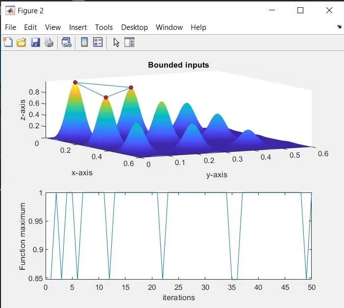
• This study is done for further optimization of the stalagmite function .
• Similar approach as first study is made and the syntax for GA is further modified and upper and lower bounds are assigned from 0-0.4 for both x and y.
• [inputs , fopt(z)] = ga(@stalagmite, 2, [],[] ,[],[],[0;0],[0.4;0.4]);
• syntax - x = ga(fun,nvars,A,b,Aeq,beq,lb,ub) , where A ,B and Aeq and beq are blanks . lb and ub represents lower and upper bounds respectively.
• It defines a set of lower and upper bounds on the design variables, x, so that a solution is found in the range lb ≤ x ≤ ub. (Set Aeq=[] and beq=[] if no linear equalities exist.)
• The rest approach is the same as study 1

Study 3 :

• Study 2 successfully optimized the function but it can still be further optimized, hence we do further one more study where we increase the ga population size by modifying the syntax for GA and set it to 270 from default 50.
• [inputs , fopt(z)] = ga(@stalagmite, 2, [], [] ,[],[],[0;0],[0;0.4],[],[],options);
• Syntax - x = ga(fun,nvars,A,b,Aeq,beq,lb,ub,nonlcon,options) minimizes with the default optimization parameters replaced by values in options. (Set nonlcon=[] if no nonlinear constraints exist.) Create options using optimoptions.
• Here values not placed are simply replaced with blank brackets .
• Again similar approach as study 1 is followed.

% case1_with_unbounded 
 for z = 1:num_case % takes values until length of num_cases
         [inputs,fopt(z)]  = ga(@stalagmite,2);% solve stalagmite function using GA and assigning to variables
         xopt(z) = inputs(1);
         yopt(z) = inputs(2);
 end
 study1_time = toc; 

 figure(1)
 subplot(2,1,1) % creates sub-plot in the figure 
 hold on
 surfc(x,y,-f) % Creates a surface
 shading interp % varies the color in each line segment and face by interpolating the colormap index or true color value across the line or face.
 plot3(xopt,yopt,-fopt,'marker','o','markersize',5,'markerfacecolor','r')% plot3 command used to plot in 3 axis
 % marker is used to create a visible points on the plot
 title('unbounded inputs') 
 xlabel('x-axis')
 ylabel('y-axis')
 zlabel('z-axis')
 subplot(2,1,2)
 plot(-fopt)
 xlabel('iterations')
 ylabel('Function maximum')

% case2_bounded_syntax
tic
 for z = 1:num_case
         [inputs,fopt(z)] = ga(@stalagmite,2,[],[],[],[],[0;0],[0.4;0.4]);
         %defines a set of lower and upper bounds on the design variables
         xopt(z) = inputs(1);
         yopt(z) = inputs(2);
 end
 study2_time = toc;

 figure(2)
 subplot(2,1,1)
 hold on
 surfc(x,y,-f)
 shading interp
 plot3(xopt,yopt,-fopt,'marker','o','markersize',5,'markerfacecolor','r')
 title('Bounded inputs')
 xlabel('x-axis')
 ylabel('y-axis')
 zlabel('z-axis')
 subplot(2,1,2)
 plot(-fopt)
 xlabel('iterations')
 ylabel('Function maximum')
 clc
 
 
 %Case3_bounded_increasing the popoulation size 
 options = optimoptions('ga');% returns a set of default options for the SolverName solver.
 options = optimoptions(options,'PopulationSize',270);%Defining population size
 
 tic
 for z = 1:num_case
         [inputs,fopt(z)]  = ga(@stalagmite, 2,[],[],[],[],[0;0],[0.4;0.4],[],[],options);
         % takes the values of options and solves ga in required population
         xopt(z) = inputs(1);
         yopt(z) = inputs(2);
 end
 Time_study3 = toc;

 figure(3)
 subplot(2,1,1)
 hold on
 surfc(x,y,-f)
 shading interp
 plot3(xopt,yopt,-fopt,'marker','o','markersize',5,'markerfacecolor','r')
 title('Increased population')
 xlabel('x-axis')
 ylabel('y-axis')
 zlabel('z-axis')
 subplot(2,1,2)
 plot(-fopt)
 xlabel('iterations')
 ylabel('Function maximum')
 
 % The Global Maximum at the position
display(inputs)

Results :

The output of the code shows three plots for unbounded, bounded, and bounded with increased population size.

Unbounded :

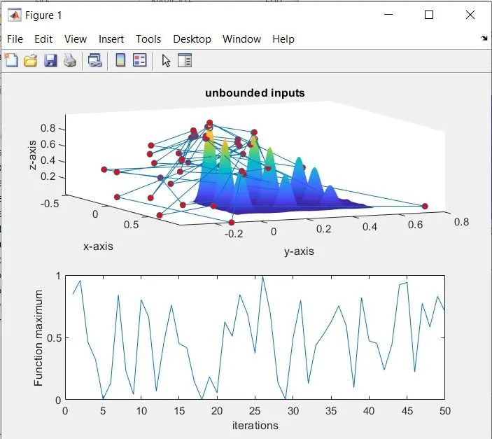
The plot shows very scattered data as it is unbounded and fitness value has failed to converge to particular point.

Bounded :

To overcome the above issue, the bounded samples method is used giving the lower and upper limits. (Therefore, it will take the
values which are greater than the upper Bound or less than the lower bound.)

Bounded with increased population size :

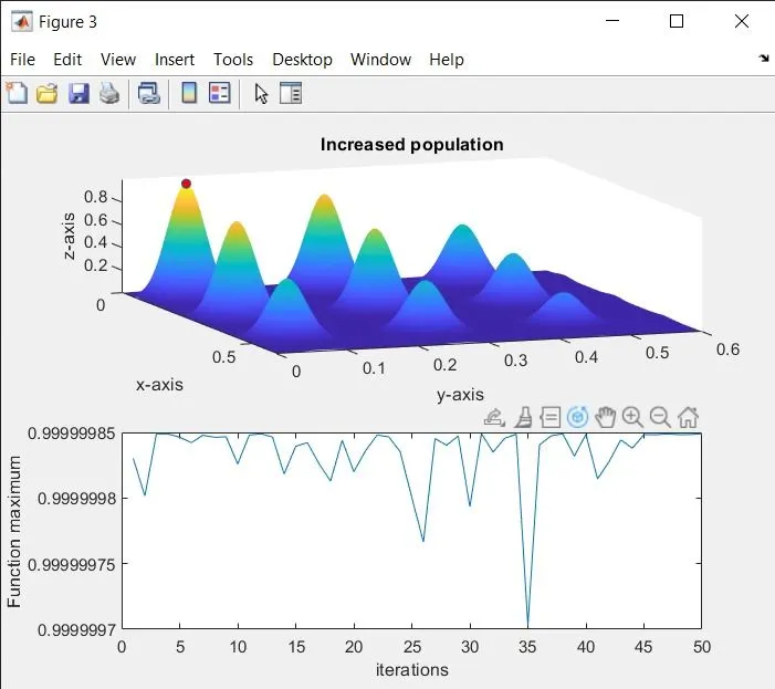
Now the above loop gives an output with different local maxima with bounded inputs. To conquer this problem, we need to increase the
population size as it increases the probability to converge to a global maximum.
The Global maximum of a function can be found by inverting the function. Find the minimum value of the inverted function,
the negative of the minimum value will give the global maximum of the function