Project 1 - Parsing NASA thermodynamic data
Aim:
Performing the file parsing for NASA thermodynamic data
Objective :
- Write a function that extracts the 14 coefficients and calculates the enthalpy, entropy, and specific heats for all the species in the data file. Note :(The FIRST 7 coefficients are HIGH-temperature coefficients and the SECOND 7 coefficients are LOW-temperature coefficients.)
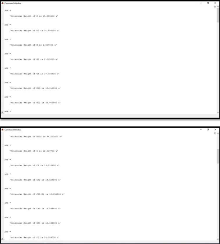
- Calculate the molecular weight of each species using the mentioned formula and display it in the command window.
- Plot the Cp, Enthalpy, and Entropy for the local temperature range (low temperature: high temperature) specific for each species.
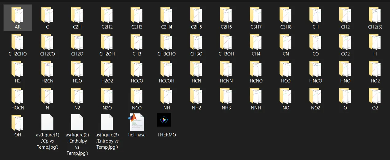
- Save the plots as images with appropriate names and dump them in separate folders for each species with a suitable name. All these should be generated automatically.
Introduction :
File parsing :
Parsing in computer languages refers to the syntactic analysis of the input code into its components parts in order to facilitate the writing of compilers and interpreters. It can be used to describe split or separation.
Parsing a file means reading in a data stream of some sort and building an in-memory model of the semantic content of that data. This aims at facilitating performing some kind of transformation on the data.
Many computational chemistry programs output text files that include a large amount of information including text and data that you need to analyze. Often, you need to sort through the output file and identify particular pieces of information that are most important to you. In general, this is called file parsing.
Thermodynamics constant :
- Specific heat :
The specific heat is the amount of heat per unit mass required to raise the temperature by one degree Celsius.
- Entropy :
Entropy, the measure of a system’s thermal energy per unit temperature that is unavailable for doing useful work. Because work is obtained from ordered molecular motion, the amount of entropy is also a measure of the molecular disorder, or randomness, of a system
In short, we can define entropy as a measure of the disorder of the universe, on both a macro and a microscopic level.
- Enthalpy:
Enthalpy, the sum of the internal energy and the product of the pressure and volume of a thermodynamic system. Enthalpy is an energy-like property or state function—it has the dimensions of energy (and is thus measured in units of joules or ergs), and its value is determined entirely by the temperature, pressure, and composition of the system and not by its history. In symbols, the enthalpy, H, equals the sum of the internal energy, E, and the product of the pressure, P, and volume, V, of the system: H = E + PV.
Molecular weight :
Molecular weight, also called molecular mass, the mass of a molecule of a substance, based on 12 as the atomic weight of carbon-12. It is calculated in practice by summing the atomic weights of the atoms making up the substance’s molecular formula.
Governing Equations :
`(Cp)/R=a1+a2*T+a3*T^2+a4*T^3+a5*T^5`
`H/(R*T)=a1+a2*T/2+a3*T^2/3+a4*T^3/4+a5*T^4/5+(a6)/T`
`S/R=a1*In*T+a2*T+a3*T^2/2+a4*T^3/3+a5*T^4/4+a7`
where,
Cp = Specific Heat (J/K kg)
H = Enthalpy (J)
S = Entropy (J/K)
R = Universal gas constant = 8.314 (J/mol.K)
T = Temperature (K)
a1...a7 = coefficients ( in the file first 7 are high temperature and other 7 are low temperature coefficients )
CODE :
clear all
close all
clc

%nasa data file parsing %
%extracting the coefficient of thermodynamics

dt=fopen('thermo.dat','r');
%readng the first 5 lines of file (not for use)
first_line = fgetl(dt); %reading the 1st line from data
global_temp = fgetl(dt) %reading 2nd line from data
temp_range = strsplit(global_temp,' ') %splitting 2nd line using blank space as delimiter
comments1 = fgetl(dt); %reading 3rd line from data
comments2 = fgetl(dt); %reading 4th line from data
comments3 = fgetl(dt); %reading 5th line from data


for i = 1:53
   % Extracting name of gas species
A = fgetl(dt); % Reading the sixth line
species = strtok(A); % Reading the species name

% Extracting co-efficient of gas species
B = fgetl(dt);
b = findstr(B,'E');
a1 = B(1:b(1)+3); % Assigning 'a' variable for the temperature co-efficients
a1 = str2num(a1);
a2 = B(b(1)+4:b(2)+3);
a2 = str2num(a2);
a3 = B(b(2)+4:b(3)+3);
a3 = str2num(a3);
a4 = B(b(3)+4:b(4)+3);
a4 = str2num(a4);
a5 = B(b(4)+4:b(5)+3);
a5 = str2num(a5);

%second line of species coefficeint
C = fgetl(dt);
c = findstr(C,'E');
a6 = C(1:c(1)+3);
a6 = str2num(a6);
a7= C(c(1)+4:c(2)+3);
a7 = str2num(a7);
a8 = C(c(2)+4:c(3)+3);
a8 = str2num(a8);
a9 = C(c(3)+4:c(4)+3);
a9 = str2num(a9);
a10 = C(c(4)+4:c(5)+3);
a10 = str2num(a10);

%third line of species coefficent
D = fgetl(dt);
d = findstr(D,'E');
a11 = D(1:d(1)+3);
a11 = str2num(a11);
a12 = D(d(1)+4:d(2)+3);
a12 = str2num(a12);
a13 = D(d(2)+4:d(3)+3);
a13 = str2num(a13);
a14 = D(d(3)+4:d(4)+3);
a14 = str2num(a14);

%Creating a vector of 500 evenly spaced temperature points
t1=200;
t2=3500;
t3=1000;
T = linspace(t1,t2,500);

%gas constant
R=8.134;

for i = 1:length(T)

 if T(i)>t3
 Cp(i) = (a1 + a2.*T(i) + a3.*T(i).^2 + a4.*T(i).^3 + a5.*T(i).^4)*R;
 H(i) = (a1 + (a2.*T(i))/2 + (a3.*T(i).^2)/3 + (a4.*T(i).^3)/4 + (a5.*T(i).^4)/5 + (a6./T(i)))*R.*T(i);
 S(i) = a1.*log(T(i)) + a2.*T(i) + (a3.*T(i)^2)/2 + (a4.*T(i)^3)/3 + (a5.*T(i).^4)/4 + a7;
 else
 Cp(i) = (a8 + a9.*T(i) + a10.*T(i).^2 + a11.*T(i).^3 + a12*T(i).^4)*R;
 H(i) = (a8 + (a9.*T(i))/2 + (a10.*T(i).^2)/3 + (a11.*T(i).^3)/4 + (a12.*T(i).^4)/5+(a13./T(i)))*R.*T(i);
 S(i) = a8.*log(T(i)) + a9.*T(i) + (a10.*T(i)^2)/2 + (a11.*T(i)^3)/3 + (a12.*T(i).^4)/4 + a14;
 end
end

mkdir(['C:\Users\ATISH\Desktop\file_parsing\',species]);

 % Plotting specific heat vs temperature
figure(1)
plot (T,Cp, 'color','b','linewidth',2)
xlabel('Temperature (K)')
ylabel('Specific Heat (J/K Kg)')
title('Specific Heat vs Temperature')
grid on


% Plotting enthalpy vs temperature
figure(2)
plot (T,H, 'color', 'r','linewidth',2)
xlabel('Temperature (K)')
ylabel('Enthalpy (J/K)')
title('Enthalpy vs Temperature')
grid on


% Plotting entropy vs temperature
figure(3)
plot (T,S, 'color', 'g','linewidth',2)
xlabel('Temperature (K)')
ylabel('Entropy (J/K)')
title('Entropy vs Temperature')
grid on

cd(['C:\Users\ATISH\Desktop\file_parsing\',species]);
saveas(figure(1),'Cp vs Temp.jpg')
saveas(figure(2),'Enthalpy vs Temp.jpg')
saveas(figure(3),'Entropy vs Temp.jpg')

% Molecular weight calculation
elements = ['H','C','O','N','A']; %  species elements vector
atomic_weight = [1.0079 12.0107 15.999 14.0067 39.948]; %  the atomic weight value of respective species
mol_wt = 0; % Declaring molecular weight to be '0'

 for l = 1:length(species)
    for m = 1:length(atomic_weight)
   if strcmp(species(l), elements(m))
    mol_wt = mol_wt + atomic_weight(m);
    position = m;
   end
 n = str2double(species(l));
 if n>1
 mol_wt = mol_wt + atomic_weight(position)*(n-1);
 end

% Printing the molecular weight of the gas species in the command window
sprintf('Molecular Weight of %s is %f',species,mol_wt)
    end
 end

end

 fclose(dt)
Explanations:
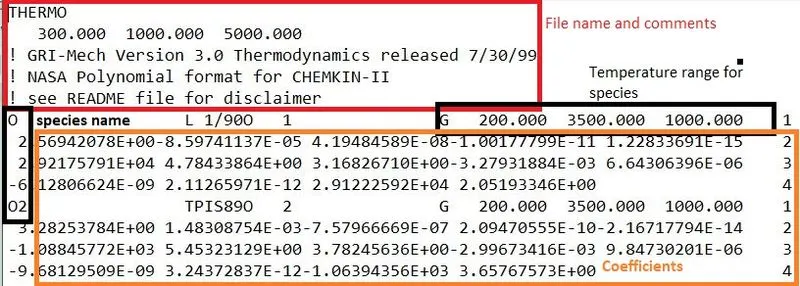
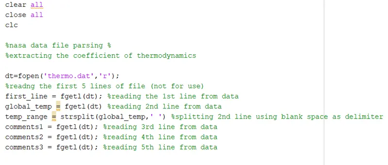
- The program begins with clear all , close all, clc which clears all the graphs, stored data previously saved.
- The code is started with opening the file using command ‘fopen(thermo.dat,r)’ ,the ‘r’ is used to read the file (we can aslo use ‘w’ which write the file).
- Next, 5 lines are includes the ‘fgetl’ command which read the each 5 lines text or integers (all the lines are stored or read n the string format). The first five seems to irrelevant as we need only the coefficient value and species name.
- Now, we will create a loop which will extract/read the species name and its coefficients value. Starting with the species name, we type fgetl(dt) nd denoting it with the variable name A. It will read the sixth line which contains the species along with the temperature range.
- Next line we use strtok which parses str from left to right, using whitespace characters as delimiters, and returns part or all of the text in species. That means we will get the all the species name under the species vector.
- Now, we are going to extract the co-efficient for the gas species in which the co-efficient locations are like in the 2 row,next 5 in the 3 row and the rest in the 4 row.
- We are going to extract these values similarly like we did for finding out the local temperatures by using the findstr and str2num commands and store it in the variables a1 to a14. For extracting we are going to locate the string ‘E’ which is present in the each co-efficient value and so it will be followed for all the co-efficients values in the same line and then we can proceed for the next lines.
- The values from a1 to a7 represent the high temperature co-efficients and the values from a8 to a14 represent the low temperature co-efficients.
- We will define the temperature as t1,t2,t3 equals to 200,3500 and,1000 respectively from which the t1 is low temperature , t2 is high temperature and t3 is mid temperature. Temperature range values from t1 to t2 is assigned using the linspace command.
- And we will define the gas constant R=8.134 .
- Again we use the for loop command is used to calculate the values of specific heat, enthalpy and entropy and the if-else command is also used to find out the required values if the temperature below the mid temperature or above the mid temperature.
- Then to create a new folder with the species we are going to use the mkdir command so that a new folder is created in the main folder.
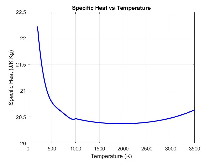
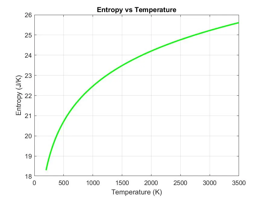
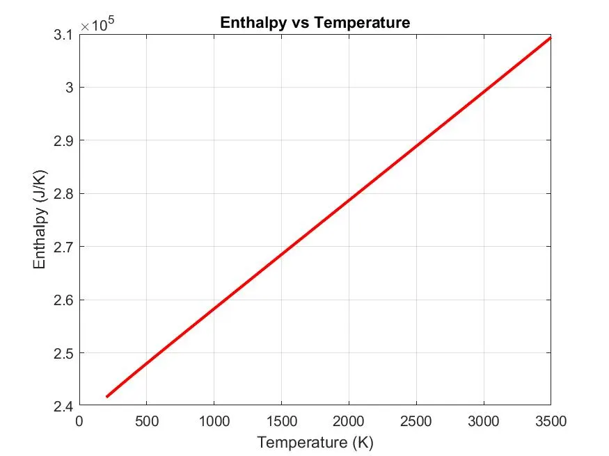
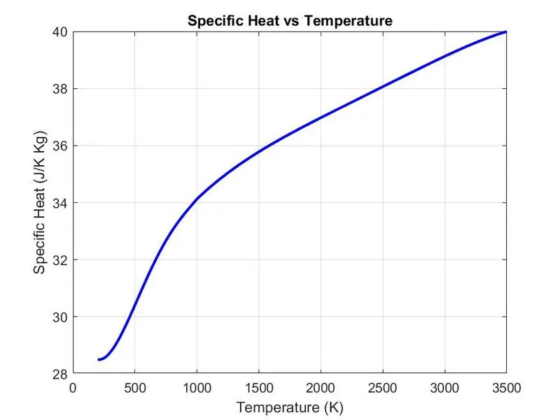
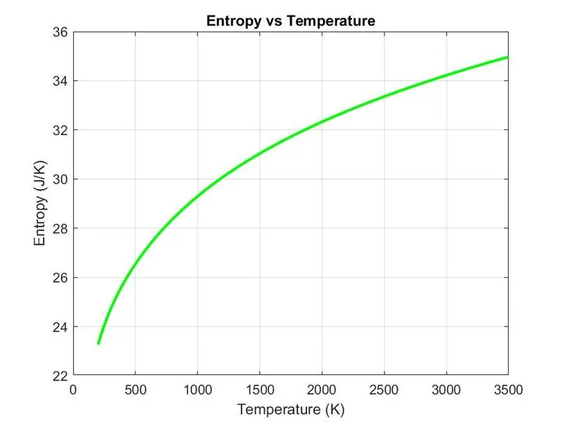
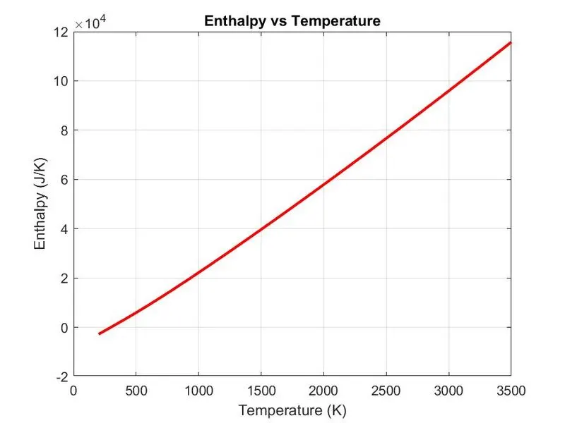
- Further, we plot the graph from the values obtained from the above step .The plots for specific heat vs temperature, enthalpy vs temperature and entropy vs temperature is plotted and the labelling of axis and the naming of the title .
- Cd command is used to change the directory to current folder mentioned and all the plots is saved in jpg format in respective species folder using saveas command.
Molecular weight calculations:
- For the molecular weight calculation we basically add the atomic weight all the species atom. In order to calculate the molecular weight of the species, we declare the species elements in the form of cell array. Their atomic mass is declared in the form of array. Then initially molecular weight is declared as zero.
- Now, for loop is used to detect if there are more than one species in the variable species. Strcmp command is used to compare and match the elements and species for further process.
- After the species name is matched and its atomic value added , it is stored under the variable name position =m .
- Sincle there can be more than two molecules of same elements, that remaining elements is calculated by first converting the species to numer using strtodouble under n variable .
- Now, if loop(n>1) is used to multiple the (n-1) to previous stored position value. Since the one molecule of element is already used the rest molecules are simply multiplied to previous by n-1.
- Towards the end we use sprintf to print the species name and its weight and all the loop is closed and followed by fclose to close the file.
Results :
O plots :
O2 plots :
Molecular weight :
values are round off:
- Molecular Weight of O: 15
- Molecular Weight of O2: 30
- Molecular Weight of H: 1
- Molecular Weight of H2: 2
- Molecular Weight of OH: 16
- Molecular Weight of H2O: 17
- Molecular Weight of HO2: 31
- Molecular Weight of H2O2: 32
- Molecular Weight of C: 12
- Molecular Weight of CH: 13
- Molecular Weight of CH2: 14
- Molecular Weight of CH2(S): 14
- Molecular Weight of CH3: 15
- Molecular Weight of CH4: 16
- Molecular Weight of CO: 27
- Molecular Weight of CO2: 42
- Molecular Weight of HCO: 28
- Molecular Weight of CH2O: 29
- Molecular Weight of CH2OH: 30
- Molecular Weight of CH3O: 30
- Molecular Weight of CH3OH: 31
- Molecular Weight of C2H: 25
- Molecular Weight of C2H2: 26
- Molecular Weight of C2H3: 27
- Molecular Weight of C2H4: 28
- Molecular Weight of C2H5: 29
- Molecular Weight of C2H6: 30
- Molecular Weight of CH2CO: 41
- Molecular Weight of HCCO: 40
- Molecular Weight of HCCOH: 41
- Molecular Weight of H2CN: 28
- Molecular Weight of HCN: 27
- Molecular Weight of HNO: 30
- Molecular Weight of N: 14
- Molecular Weight of NNH: 29
- Molecular Weight of N2O: 43
- Molecular Weight of NH: 15
- Molecular Weight of NH2: 16
- Molecular Weight of NH3: 17
- Molecular Weight of NO: 29
- Molecular Weight of NO2: 44
- Molecular Weight of HCNO: 42
- Molecular Weight of HOCN: 42
- Molecular Weight of HNCO: 42
- Molecular Weight of NCO: 41
- Molecular Weight of CN: 26
- Molecular Weight of HCNN: 41
- Molecular Weight of N2: 28
- Molecular Weight of AR: 39
- Molecular Weight of C3H8: 44
- Molecular Weight of C3H7: 43
- Molecular Weight of CH3CHO: 43
- Molecular Weight of CH2CHO : 42
Conclusion :
We have successfully parsed/extracted the coefficient value of each species from the NASA thermodynamic file and plotted the respective species graph for the specific heat, entropy and enthalpy followed by which we calculated the molecular mass also.
References :
https://in.mathworks.com/help/matlab/ref/strtok.html
https://in.mathworks.com/help/matlab/ref/mkdir.html